Sensing deep-ocean temperatures

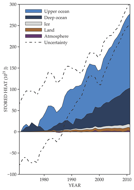
Changes in the concentration of greenhouse gases in our atmosphere affect the thermal-energy balance in Earth’s climate system. But thanks to its huge volume, deep basins, and large heat capacity, the global ocean has largely forestalled atmospheric warming by acting as a heat sink. Indeed, the ocean stores more than 90% of the excess heat Earth has accumulated since 1971. Compare that with the scant 1% stored in the atmosphere, as shown in figure 1.

The ocean also redistributes the absorbed energy around the planet. Colder and thus denser waters from high latitudes can sink from the surface and spread toward the equator beneath warmer, lighter waters at lower latitudes. In the northern North Atlantic Ocean and the Southern Ocean around Antarctica, water is cooled so much that it can sink to great depths, where it then spreads out to fill much of the rest of the deep ocean. As surface waters warm, so do those sinking waters, which increase the temperature of the ocean interior much more quickly than would the downward mixing of warmer layers with colder ones (see the article by Adele Morrison, Thomas Frölicher, and Jorge Sarmiento, Physics Today, January 2015, page 27 ). The large-scale transport of water, heat, and salt in distinct density ranges, called the meridional overturning circulation, is a key part of climate studies. ¹

Because the ocean is the largest heat reservoir in the climate system, accurately measuring its temperature changes is necessary to understand the evolution of the climate and guide environmental policy. That’s a daunting task, though: Distances are huge, access is limited, ships are slow and expensive, and point-temperature measurements—the traditional method for the job—cannot easily distinguish local short-term temperature fluctuations from the actual climate signal, which is generally far smaller. Because those fluctuations are pervasive—typically caused by mesoscale current eddies hundreds of kilometers wide and by internal waves triggered by current flow over a sloping seafloor—temperature surveys must be averaged out by multiple measurements in space and time.

In one of the most impressive achievements of the past couple of decades, oceanographers in 2001 initiated an oceanic observing system known as the Argo program (see Physics Today, July 2000, page 50 ). Today its global array of 3900 robotic floats can directly and repeatedly sense temperature (to within 0.002 °C), pressure, salinity, and ocean circulation. ² Over the course of 10-day dive cycles, the floats adjust their buoyancy to record data at depths between 2000 m and the surface, where they transmit their GPS location to a satellite. An international collaboration sustains the Argo program data and controls all stages of the operation, from refurbishment or replacement of each float every 3–5 years to data control, archiving, and dissemination.

In 2005 the program achieved worldwide ocean coverage—at least over ice-free regions—with the floats spaced about every 3° of longitude and latitude. Its data reveal a global average warming trend of about 0.11 °C per decade near the ocean’s surface. That trend decreases with depth: The warming drops to about 0.04 °C per decade around 200 m, and to less than 0.02 °C per decade around 500 m. ¹ However, as oceanographer Dean Roemmich and his colleagues showed last year, those relatively shallow measurements underestimate the total oceanic heat content. ² To better estimate the heat uptake, comprehensive measurements must be made down to at least 4000 m, a depth representing 90% of the total ocean volume.

Getting deep

Below 4000 m, temperature variations are expected to be significantly smaller than they are near the surface. That makes them more challenging to resolve. Those depths are also far out of reach of today’s Argo floats. Fortunately, the success of the Argo program has spurred an effort, now under way, to develop floats that can withstand greater pressures and continuously sample ocean temperatures and salinities down to 6 km. Goals include achieving a better assessment of the excess heat stored in the global ocean and estimating the decadal variability in deep-ocean temperature and circulation patterns. ³

To date, only sparse repeated measurements of deep-ocean temperatures are available—primarily from a few dozen ship-based research expeditions that conduct coast-to-coast hydrographic surveys every decade or so. ⁴ Such direct ship-based measurements have shown decadal changes, notably in the Southern Ocean, but the measurements are so scarce that what happens at shorter time scales between surveys remains unclear. In 2010 University of Washington oceanographers Sarah Purkey and Gregory Johnson used ship-based temperature measurements with an accuracy of about 0.002 °C to estimate the temperature trends in deep basins. ⁵ They concluded that the ocean below 4000 m was storing heat at the rate of about 0.03 W/m ² , applied over the whole Earth. That rate amounts to about 5–7% of the global imbalance estimated this past year from Argo observations of the upper ocean.

A more global method for estimating deep-ocean heating is to use satellite altimetry to measure sea-level rise and gravity-field measurements of ocean mass (see the article by Bruce Douglas and Richard Peltier, Physics Today, March 2002, page 35 ). By the thermosteric effect, water expands as it warms and contracts as it cools. Hence the sea-level rise caused by deep-ocean heating can be estimated by subtracting the amount of sea-level rise caused by melting land ice and upper-ocean expansion, as indicated by the Argo floats, from the total amount of sea-level rise measured by satellites. Such an indirect method, however, contains its own uncertainties.

Acoustic thermometry

Sound is a natural way to probe the ocean because it can propagate long distances with little attenuation and at a speed $c$ that is sensitive to the local properties of seawater—temperature $T$, salinity $S$, and pressure. ^{6 , 7} At any given depth, the speed of sound increases in warmer water and decreases in cooler water. As currently practiced, acoustic thermometry thus consists of measuring the travel times of sound pulses between a fixed source and a receiver and then interpreting those times in terms of the sound speed and temperature.

To first order, the sound speed $c$ in m/s follows a simple empirical formula: $c=1449+4.6T+(1.34-0.01T)(S-35)+0.016z$, in which $T$ is measured in celsius, $S$ is a unitless quantity derived from conductivity and temperature measurements, $z$ is in meters, and the last, depth-dependent term embodies density and static-pressure effects. In the ocean, the effects of density are generally ignored, and currents are slow compared with the speed of sound. The ocean’s sound-speed profile as a function of depth results from the competition between the temperature term, which dominates near the surface, and the pressure term, which dominates as depth increases. At Earth’s midlatitudes, $c$ decreases with depth until it reaches a minimum at about 1000 m and then increases with pressure, as illustrated in the box on page 35. That sound-speed profile influences sound propagation by refracting the wavefronts toward the minimum—referred to as the axis of the sound fixing and ranging (SOFAR) channel. By analogy to geometric optics, the path that sound follows, known as a ray, is normal to its wavefront.

The SOFAR channel thus acts as a natural waveguide in which sound becomes trapped, oscillates about the sound-speed minimum, and propagates for potentially thousands of kilometers (see reference 6 and the article by Bill Kuperman and Jim Lynch, Physics Today, October 2004, page 55 ). Sounds produced in the ocean travel in all directions, just as they would in free space. That means that a sound pulse splits up into many rays, and the rays reaching a distant receiver will each have travelled along its own unique path. The rays also arrive at different times. A ray traveling from an acoustic source at a steeper angle relative to the SOFAR axis samples a larger swath of the water column than does a ray traveling at a shallower angle. And because the deeper and shallower waters encountered by the steeper rays increase their speed beyond what’s needed to make up for the longer path lengths, they arrive earlier, as illustrated by the magenta and green rays in the box figure.

Model and measurement

The travel time of a sound pulse along a particular ray path is given by ${\int }_{\gamma }\mathit{ds}/c(s)$, where $\gamma$ is the curved path, $c\left(s\right)$ is the sound speed along it, and $\mathit{ds}$ is the incremental arc length. In practice, for source–receiver separations greater than about 100 km, rays are identified by their arrival times and incidence angles at an array of hydrophones. Indeed, measuring the ray arrival-time structures between several source–receiver pairs distributed around a given volume of ocean can provide multiple perspectives of sound-speed variations. ⁷

Provided that a sufficiently accurate numerical model of sound propagation in the ocean is available to simulate the rays’ arrival times for a given set of sources, receivers, and sound-speed variations, the patterns of arrival times predicted from the simulation can be compared with experimental measurements. If an unambiguous matchup is found, then the predicted ray arrival times can be used to solve the inverse problem: calculating adjustments to the sound-speed estimate from the differences between simulated and observed arrival times. ⁷ Hence by adjusting the sound speeds, instrument positions, and timing offsets—that is, discrepancies between starting times of broadcast and receiver clocks—in the numerical simulations, one can find a best fit of the predicted parameters to observations. Temperature variations can then be inferred from the estimated sound-speed variations using the known relationships between them.

Because rays in the ocean oscillate above and below the sound channel axis (see the box), their measured arrival times are sensitive to sound-speed variations over a broad, generally three-dimensional region. Each measurement thus represents a weighted average of those variations along a ray’s path. That’s both an advantage and a disadvantage for reconstructions of ocean temperature changes. On the one hand, the spatial averaging reduces the effects of variability from internal waves and eddies because small-scale perturbations tend to average out. On the other hand, it worsens the problem of locating the perturbations. Only a diversity of sampling methods that don’t average regions above and below the SOFAR axis can eliminate that ambiguity. As early as 1979, oceanographers Walter Munk and Carl Wunsch proposed that acoustic travel-time data could be combined with satellite altimetry to monitor the world’s oceans. ⁸

Manmade sources

Beginning with an experiment in 1826, when a bell was rung in the waters of Lake Geneva, Switzerland, oceanographers have made their own sources of sound, commonly referred to as active sources, to measure sound speeds underwater. For ranges greater than 100 km, they deploy transducers that emit high-bandwidth signals at frequencies lower than 400 Hz. Sound attenuation and scattering generally decrease as the frequency decreases; the longer the range, the lower the required frequency.

In 1960, explosives dropped into the water off a ship near Perth, Australia, created sound pulses that were recorded at a hydrophone off the coast of Bermuda, halfway around the world. In that case, only three measurements were made, which complicated the scientists’ interpretation of the results. ⁷ After ocean eddies were later discovered, Munk and Wunsch proposed a system of moored sources and receivers that allowed them and other oceanographers to repeatedly survey particular regions using a network of crossing acoustic paths. To reconstruct a time-evolving 3D sound-speed field, they used a method they called acoustic tomography—an analogue of medical tomography—in which receivers map not the attenuation of x rays but the travel times of acoustic signals between fixed points on the periphery of an ocean basin. The travel times are then inverted to yield sound speeds. ⁷

A large (and expensive) amount of energy is needed to produce the low-frequency signals required for such experiments. That makes it difficult for battery-powered sources moored underwater to transmit as loudly or as often as desired; cabled sources, by contrast, can exploit land power but are many times more expensive to deploy. Concerns about ocean noise pollution—in particular, its effects on marine mammals—have also proven to be a constraint on experiments.

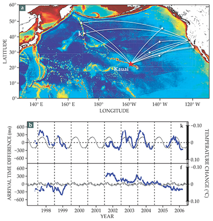
Nonetheless, several experiments have borne out the acoustic tomography—and by extension thermometry—concept. Figure 2 outlines one of them: a 9-year project to monitor temperature fluctuations in the northern Pacific Ocean. ⁹ Reassuringly, the measured (blue) and simulated (gray) temperature variations are comparable and, where paths sample the northernmost part of the ocean, closely follow seasonal changes.

Because the number of possible measurements of the ocean’s interior grows as the product of the number of sources and the number of receivers, relatively few instruments are required—at least compared with the number needed for conventional point measurements. Moreover, because acoustic thermometry inherently samples a broad, 3D swath of ocean, it automatically provides a spatial average difficult to achieve with a large number of point measurements and potentially at a far higher temporal resolution. Even so, the high cost of existing hardware and limited funding have stymied efforts to deploy a global network of sources and receivers.

Ambient noise

The ocean environment is filled with natural noises—surface winds, earthquakes, and breaking ice among them—in addition to manmade noises from ship engines and offshore platforms. One can therefore ask whether such ambient noises can replace active underwater transducers as sources for acoustic thermometry. Indeed, a rapidly emerging research field has proven that a Green’s function—by definition, the response to an impulsive source—can be extracted from random noise fields (see the article by Roel Snieder and Kees Wapenaar, Physics Today, September 2010, page 44 ). Already a standard methodology in seismology and helioseismology, ambient-noise imaging is rapidly expanding to such other applications as nondestructive testing, medical ultrasonics, and ocean acoustics. Basically, the cross correlation of random noise recorded at two receivers yields a set of time delays associated with the ray travel times between those receivers, just as if one of them was acting as a transmitter of the signal.

The method was first demonstrated for ocean acoustics 12 years ago over relatively short ranges of less than 10 km between the receivers. ¹⁰ What limits it for longer, basin-wide distances is the relatively short time scale—minutes to hours—of the ocean’s sound-speed fluctuations, compared with the averaging time—from days to weeks—required to extract arrival times from the ambient-noise correlation. Fortunately, the last-arriving and most energetic ray that reaches the receivers is an unusually stable acoustic feature because it corresponds to trapped sound propagating nearly horizontally over long distances along the SOFAR channel.

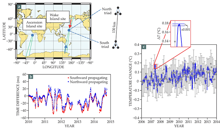
Last year two of us (Sabra and Kuperman) took part in a study demonstrating the feasibility of measuring temperature variations by correlating noise signals that originated from Earth’s polar regions and were detected at two sites, each with two receiver arrays. ¹¹ The study used continuous recordings of low-frequency (roughly 10 Hz) ocean noise at hydrophones that are currently part of the Comprehensive Nuclear-Test-Ban Treaty’s network of hydroacoustic stations, whose principal purpose is to monitor nuclear explosions (see the article by Matthias Auer and Mark Prior, Physics Today, September 2014, page 39 ). We and our colleagues processed the low-frequency noise once each week for seven years and translated the variations in signal arrival times into temperature variations.

The results, shown in figure 3, confirmed that ambient-noise thermometry is sufficiently accurate to detect mesoscale variations of ocean temperatures occurring within the effective depths of the SOFAR channel—about 400–1500 m at the chosen sites. As expected, different ocean basins exhibit different warming trends due to the complex redistribution of heat through global circulation paths. For instance, unlike the temperature estimates obtained near Wake Island in the Pacific Ocean, which showed little long-term change, those obtained near Ascension Island in the Atlantic Ocean exhibited a clear warming trend of 0.013 ± 0.001 °C/yr over the eight years measurements were taken there. The same magnitude trend was borne out by averages from the Argo floats in that area. ^{11 , 12}

Toward integration

Establishing a global ocean observing system is paramount to accurately determining worldwide heat distribution in the ocean, the largest heat reservoir for Earth’s climate. The success of the Argo program and the ongoing development of its extension to deeper waters sets a clear path toward that goal. Studies of acoustic thermometry demonstrate that it offers complementary estimates of ocean temperatures, especially in ice-covered regions where direct access is difficult. Moreover, the acoustic method probes larger volumes of water with higher temporal resolution—down to a scale of tens of minutes, compared with interpolated point measurements from floats, which currently require 10 days or more.

The advantages and applicability of acoustic methods are likely to grow as the technology improves, installation costs decrease, and receiver networks expand. Indeed, hardware improvements may eventually foster the integration of remote acoustic measurements and free-drifting floats. One can imagine, for instance, a global network of free-drifting floats that are outfitted not only with temperature, pressure, and salinity sensors but also with hydrophones.

Box. Ocean sound propagation

The speed of sound in the ocean increases with increasing temperature, salinity, and pressure. Near the ocean surface, temperature dominates; as temperature falls with depth, so does sound speed, as shown in the figure’s left-hand panel. At greater depths, temperature becomes nearly constant. Pressure then dominates, and sound speed rises with depth as pressure does. The result is a sound-speed minimum, known as the sound channel axis, about 1000 m deep at midlatitudes.

The ocean is typically modeled as an acoustic waveguide with a variable sound speed $c(\mathbf{r},z)$ whose value depends on the horizontal position vector $\mathbf{r}$ and depth $z$. For a formal description of sound propagation, one turns to the Helmholtz wave equation

$$\left[{\nabla }^2+\frac{{\omega }^2}{c^2(\mathbf{r},z)}\right]P(\mathbf{r},z,\omega )=F({\mathbf{r}}_{\mathrm{s}},z_{\mathrm{s}},\omega ),$$

which can be solved for arbitrary sound-speed variations. ⁶ In that equation, $P$ denotes the received pressure field at a hydrophone from a broadcast signal $F$ at horizontal position ${\mathbf{r}}_{\mathrm{s}}$, depth $z_{\mathrm{s}}$, and frequency $\omega$.

Much insight can be gained from approximations in which the wave equation is solved for a set of range segments between source and receiver, with each segment having a depth-dependent sound-speed profile. Separation of variables $\mathbf{r}$ and $z$ for each of those local segments yields a range-independent but depth-dependent equation that is analogous to the equation for a quantum mechanical potential well, in which the sound-speed profile acts as the well. The analogy is particularly evident when the shape of the region around the sound-speed minimum is approximated as quadratic. The resulting oscillatory parts of the eigenstates determine sound trajectories and spread out in space in exact analogy to the eigenstates of a simple harmonic oscillator.

The right-hand panel of the igure shows that sound follows ray-like trajectories through the ocean with turning points in the water column determined by Snell’s law of refraction. The ocean’s local acoustic refractive index is $c(\mathbf{r},z)/c_0$, where $c_0$ represents the ocean’s nominal sound speed of 1500 m/s. In the range-independent case, Snell’s law is nothing more than a statement of conservation of horizontal wavenumber. The horizontal wavenumber for a given ray is defined as the projection of the wavenumber vector $\mathbf{k}$, which points in the ray’s direction with a magnitude $\left|\mathbf{k}\right|=\omega /c(\mathbf{r},z)$, onto the horizontal axis.

Sound can therefore propagate along a waveguide centered on the sound-speed minimum without interacting with the surface or seafloor. The conservation law dictates that a ray bends toward lower speed and cycles between the depths of its turning points. A ray (magenta) that follows a steeper angle and samples a greater range of depths reaches a hydrophone earlier than one (green) launched at a shallower angle and that hews more closely to the waveguide’s axis. If the ocean warms up between a sound source and a receiver, the travel times for both rays decrease, as shown in the bottom panel. (Figure adapted from J. Howard, Scripps Institution of Oceanography Explorations 5, 2, Fall 1998.)

References

1. R. K. Pachauri et al., eds., Climate Change 2014: Synthesis Report. Contribution of Working Groups I, II, and III to the Fifth Assessment Report of the Intergovernmental Panel on Climate Change, IPCC, 2014).
2. D. Roemmich et al., Nat. Clim. Change 5, 240 (2015). https://doi.org/10.1038/nclimate2513
3. G. C. Johnson, J. M. Lyman, Nat. Clim. Change 4, 956 (2014). https://doi.org/10.1038/nclimate2409
4. J. P. Abraham et al., Rev. Geophys. 51, 450 (2013). https://doi.org/10.1002/rog.20022
5. S. G. Purkey, G. C. Johnson, J. Clim. 23, 6336 (2010). https://doi.org/10.1175/2010JCLI3682.1
6. F. B. Jensen et al., Computational Ocean Acoustics, 2nd ed., Springer, 2011).
7. W. Munk, P. Worcester, C. Wunsch, Ocean Acoustic Tomography, Cambridge U. Press (2009).
See also H. Medwin, Ocean Acoustic Tomography Sounds in the Sea: From Ocean Acoustics to Acoustical Oceanography, Cambridge U. Press, 2005).8. W. Munk, C. Wunsch, Philos. Trans. R. Soc. London A 307, 439 (1982). https://doi.org/10.1098/rsta.1982.0120
9. B. D. Dushaw et al., J. Geophys. Res. Oceans 114, C07021 (2009). https://doi.org/10.1029/2008JC005124
10. P. Roux, W. A. Kuperman, NPAL Group, J. Acoust. Soc. Am. 116, 1995 (2004). https://doi.org/10.1121/1.1797754
11. K. F. Woolfe et al., Geophys. Res. Lett. 42, 2878 (2015). https://doi.org/10.1002/2015GL063438
12. X. Chen, K.-K. Tung, Science 345, 897 (2014). https://doi.org/10.1126/science.1254937
More about the authors
Karim Sabra is an associate professor in the school of mechanical engineering at the Georgia Institute of Technology in Atlanta. Bruce Cornuelle is a researcher and Bill Kuperman is a professor, both at the Scripps Institution of Oceanography in La Jolla, California.