Relativistic quantum chaos in graphene
DOI: 10.1063/PT.3.4679


In his 1987 best seller Chaos: Making a New Science, science journalist James Gleick wrote, “Where chaos begins, classical science stops.” Indeed, after relativity and quantum mechanics, chaos became the 20th century’s third great revolution in physical sciences. Chaos results from the sensitivity of a nonlinear system to initial conditions, and it makes classical evolution appear random with time (see the article by Adilson Motter and David Campbell, Physics Today, May 2013, page 27 ). That sensitivity is the origin of Edward Lorenz’s well-known butterfly effect 1 —named for the idea that a butterfly flapping its wings in South America could set off a tornado in Kansas—which rules out any hope for long-term weather forecasting.
Chaotic behavior manifests in quantum and relativistic systems, and classical chaos can lead to new manifestations in systems that are both relativistic and quantum mechanical—such as graphene, whose electrons can behave like massless particles. Those novel fingerprints of chaos are of theoretical and practical interest.
Classical chaos emerges in, for example, classical particles bouncing around elastically, similar to a billiard ball. For a billiard system with the usual rectangular boundary, two nearby particles with the same momentum reflect off the boundary with equal momentum. But when the boundary is curved, the reflected momenta of the particles are different, sometimes drastically so. That sensitivity to momentum provides the nonlinearity required for chaos in a simple system geometry, such as an oblong shape that resembles a sports stadium.
Classical light rays imitate a billiard system when confined in a cavity. To produce confinement, the cavity’s refractive index must be larger than that of the surrounding medium, so that the rays undergo total internal reflection for angles larger than the critical angle, which is determined by the ratio of the cavity to exterior refractive indices. Unlike the billiard system, however, light rays can escape from the cavity when their incident angle is less than the critical angle.
Figure
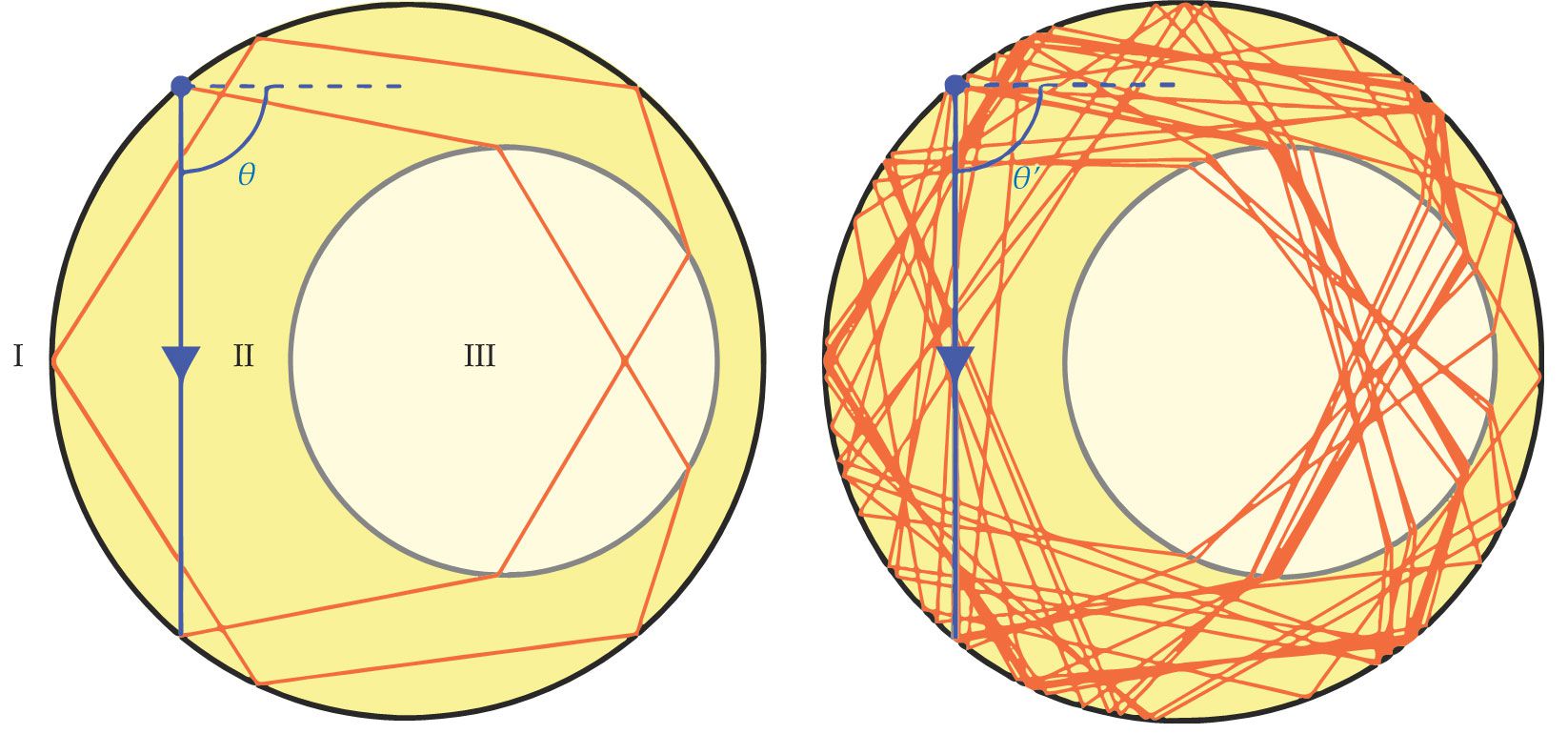
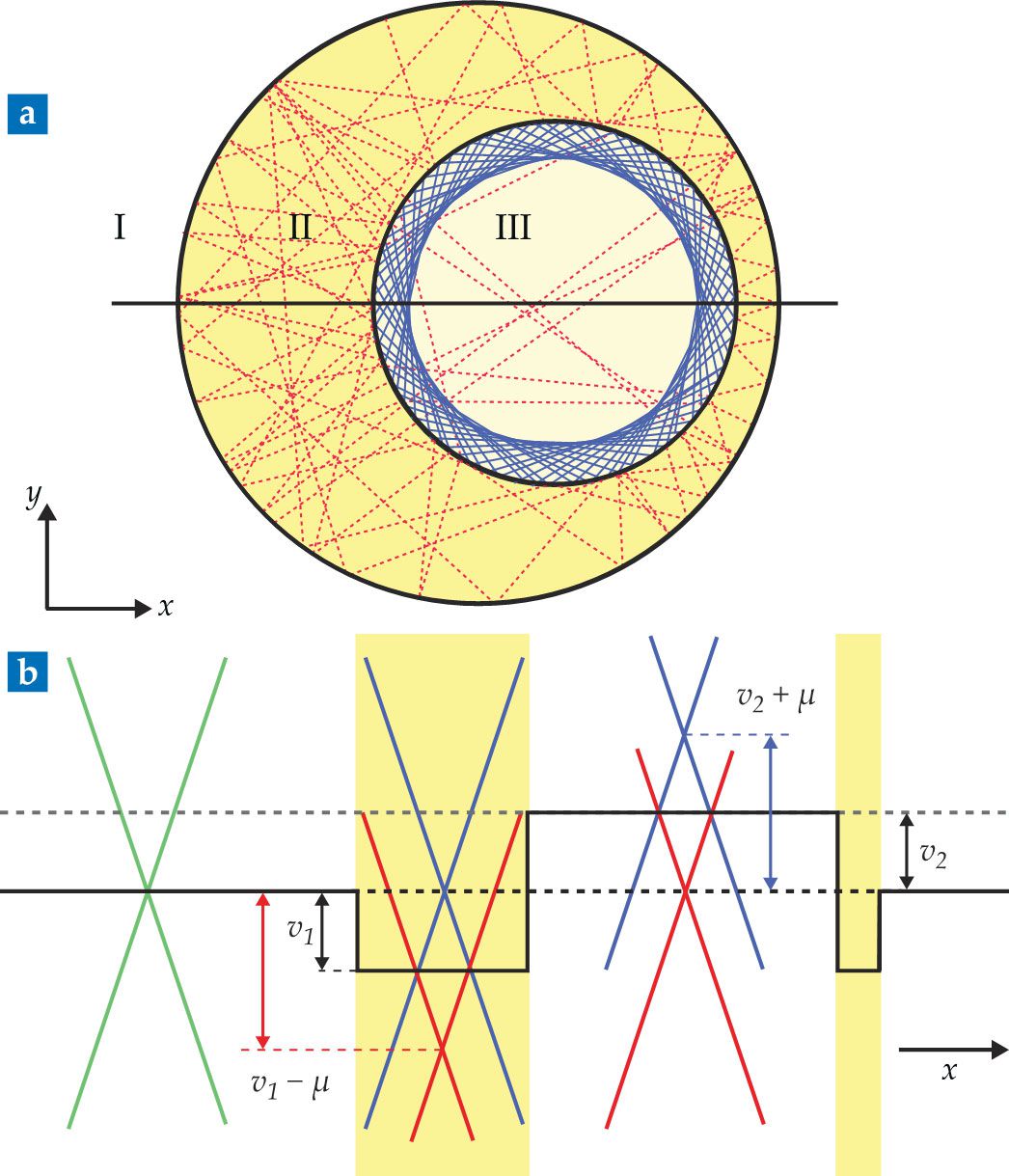
Figure 1.

Light trapped in this cavity displays chaotic behavior. In this dielectric medium the index of refraction is largest in the smallest circle (region III), smaller in the region between the two circles (region II), and smallest in the surrounding area (region I). Two ray trajectories (blue arrows) differ only slightly in their initial angles,
It’s all relative
The analogy between classical particles in a billiard system and light rays in a dielectric cavity raises the question of relativity’s role. Although both share many features, the particles are nonrelativistic whereas light is relativistic. The difference between them is best described by the dispersion relation, which gives the relationship between the energy and momentum. For a nonrelativistic particle, the energy is proportional to the momentum squared, but for a photon with zero rest mass, the energy is linearly proportional to the momentum.
In quantum mechanics, nonrelativistic particles are described by the Schrödinger equation, which has a quadratic dispersion relation. Relativistic particles, on the other hand, are typically described by the Dirac equation, and for a massless relativistic particle, the dispersion relation is linear. The Schrödinger equation also doesn’t include the spin, which is naturally embedded in the Dirac equation.
What happens when quantum mechanical systems are chaotic? The fundamental equations for such systems—Schrödinger or Dirac—are linear and thus rule out real chaotic behavior. As Michael Berry stated in 1989, “There is no quantum chaos, in the sense of exponential sensitivity to initial conditions, but there are several novel quantum phenomena which reflect the presence of classical chaos.”
2
Nevertheless, the somewhat inaccurate term “quantum chaos” has taken root to describe the manifestations or fingerprints of classical chaos in a quantum system.
3
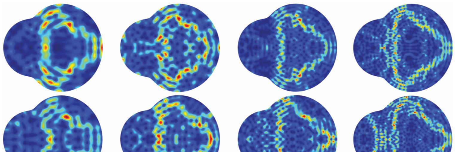
In stadium billiards, for example, a classical particle will go through almost every point in the system in the course of evolution, with equal probability of being at any one point. But in quantum mechanics, the wavefunctions concentrate on some unstable classical periodic orbits—so-called quantum scars, shown in the opening image on

The probability (red high, blue low) that an electron is in any given spot in a chaotic Dirac system forms patterns called quantum scarring. (Adapted from ref.
In the past 15 years, researchers have developed and studied so-called Dirac materials, which host quasiparticles that behave according to the Dirac equation. The most common such material is graphene, a one-atom-thick layer of a hexagonal lattice of carbon atoms. 4 , 5 After the successful isolation of a single layer of graphene 4 in 2004, researchers have prepared a variety of two-dimensional solid state materials (see the article by Pulickel Ajayan, Philip Kim, and Kaustav Banerjee, Physics Today, September 2016, page 38 ), whose quasiparticles’ energy exhibits a linear dependence on momentum. As a result, 2D Dirac materials are described by relativistic quantum mechanics. With available Dirac materials, a viable field has emerged: relativistic quantum chaos, 6 which seeks to discover, understand, and exploit fundamental phenomena arising from the interplay between chaos and relativistic quantum mechanics.
Get to the (Dirac) point
Albert Einstein’s theory of special relativity says that a massless particle such as a photon has energy proportional to its momentum, with the speed of light as the proportionality constant. Similarly in graphene and other Dirac materials, quasiparticles have a linear relationship between their energy
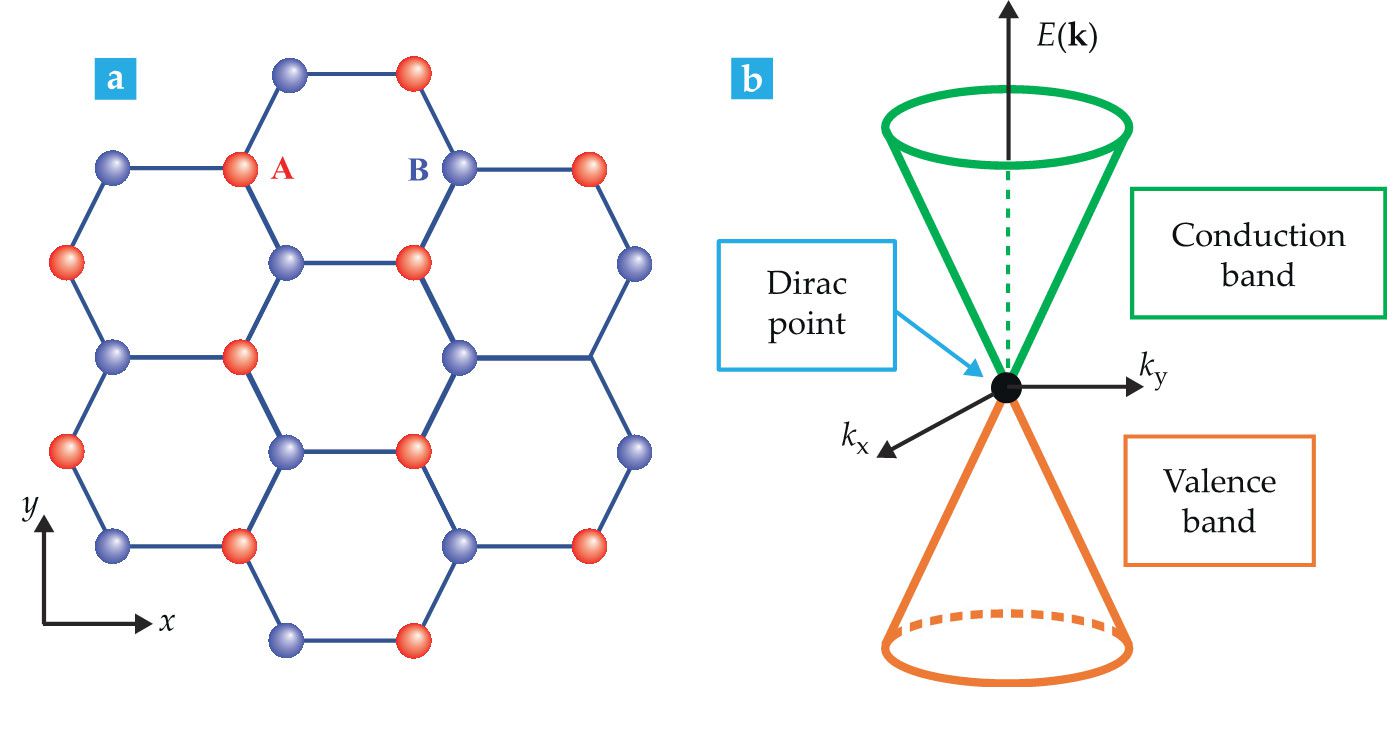
Graphene’s linear dispersion relation is a product of the lattice’s geometry and the resulting band structure. Graphene is a honeycomb lattice with two nonequivalent atomic sites in each unit cell, so the entire lattice can be regarded as two triangular lattices, A and B, as shown in figure
Figure 2.

Graphene’s lattice determines the energy band structure. (a) The two-dimensional honeycomb lattice comprises two nonequivalent triangular sublattices, A (red) and B (blue), of carbon atoms. (b) That structure determines the relation between an electron’s energy
Graphene and other 2D Dirac materials possess a unique quantum number called the pseudospin degree of freedom. 4 , 5 The two nonequivalent atomic sites, A and B, provide two independent types of quasiparticle motion. Because the quasiparticles can occupy either A or B, they are said to have pseudospin-½ in addition to the usual real spin-½ (up or down). Without an external magnetic field, the pseudospin Dirac cones are degenerate in the real spin, but in the presence of a magnetic field, the spin degeneracy is broken by the interaction between the field and the real spin.
Because of their shared linear dispersion relation, Dirac fermions behave in a way that is analogous to photons’ behavior in optics; reframing relativistic quantum mechanical phenomena in terms of optics is known as Dirac electron optics. For example, Snell’s law can predict the behavior of a graphene sheet with a potential difference
Chaotic graphene
To introduce chaos in a relativistic quantum system, a graphene sheet can mimic the optical cavity from figure
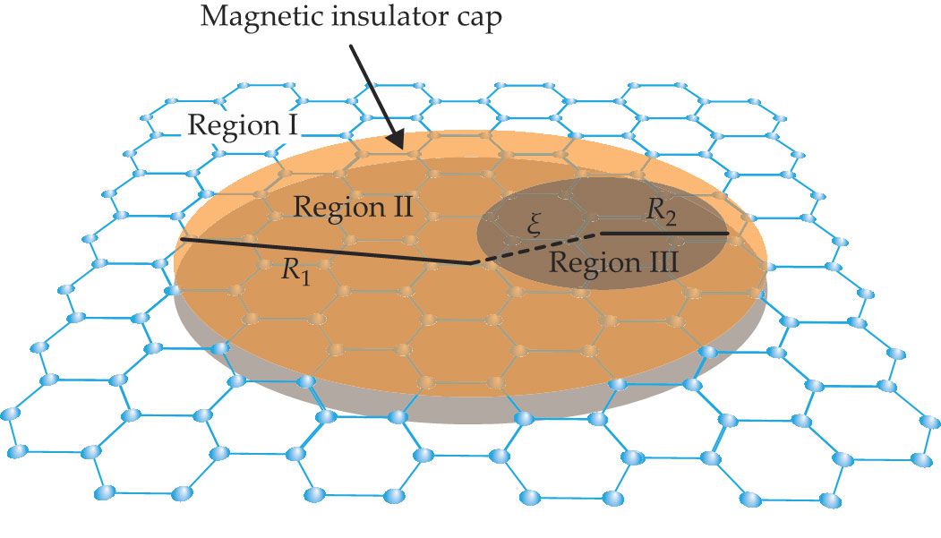
Figure 3.

A graphene-scattering system analogous to the optical cavity in figure
Figure
Figure 4.

Relativistic quantum chaos emerges in the graphene device shown in figure
Figure
That energy landscape can be reframed in terms of the effective refractive index for the electrons in regions II and III:
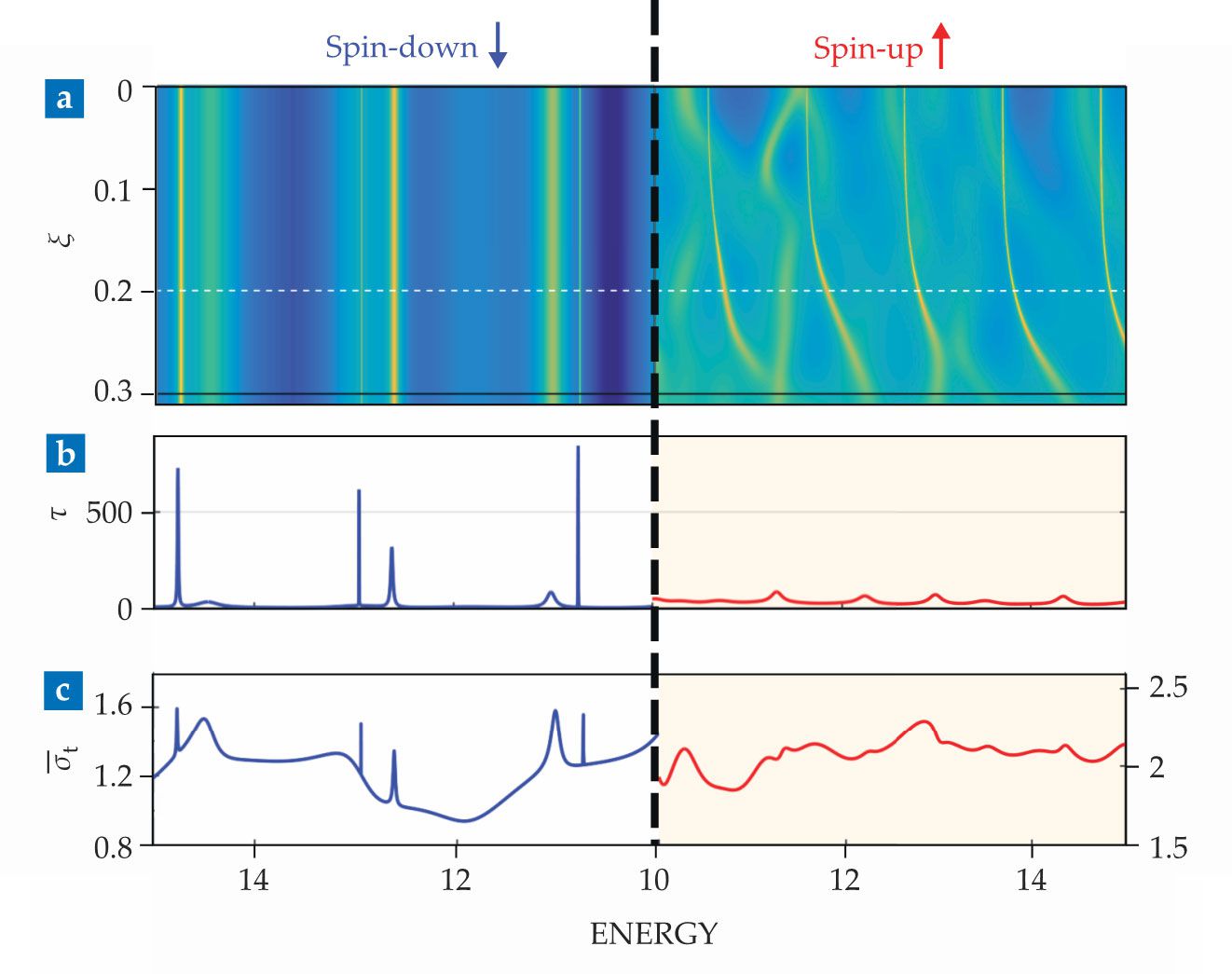
The two different types of classical dynamics lead to distinct relativistic quantum manifestations for spin-up and spin-down electrons, as illustrated by the differences between the graphs on the left and right of figure
Figure 5.

Spin-up and spin-down electrons manifest different classical behavior for the system in figure
Relativistic tunneling
In the past decade, researchers have investigated, mainly theoretically and somewhat experimentally, many topics in relativistic quantum chaos, 6 including relativistic quantum scars, Klein tunneling, superpersistent currents in chaotic Dirac rings, the interplay between chaos and spin, and the suppression of chaos in systems with spin-1 and pseudospin-1. Here, we have presented one concrete phenomenon: spin-dependent, coexistent regular and chaotic scattering. The phenomenon is counterintuitive from the perspective of nonrelativistic quantum chaos: Nonrelativistic quantum particles can’t penetrate a potential barrier with probability one, as graphene’s electrons do.
That unique phenomenon in relativistic quantum mechanics is called Klein tunneling—named for Oskar Klein, who first discovered the underlying physics in 1929 while studying the scattering of electrons based on the Dirac equation. 11 In general, a particle’s wave nature enables the electrons to pass through a classically forbidden region with a finite probability. That tunneling effect is fundamental to quantum mechanics and has significant applications in quantum computing and sensing. In nonrelativistic quantum systems, the tunneling probability typically decreases exponentially with the potential barrier’s height and width. But in relativistic quantum mechanics, the linear dispersion relation can allow particles with an internal degree of freedom, such as spin or pseudospin, to penetrate unimpeded through a high and wide potential barrier.
Klein tunneling has been observed experimentally in, for example, graphene and photonic crystals, but it’s a somewhat controversial issue with no one accepted model to explain it. For 2D Dirac materials, one explanation for the physical origin of the phenomenon is the charge of the quasiparticles. For a Fermi energy above the Dirac point in figure
Another way to understand Klein tunneling is through chirality. A massless quasiparticle in a Dirac material possesses a quantum number, known as chirality, which is the projection of its pseudospin in the direction of its momentum. Pseudospin is locked with momentum, so backscattering at normal incidence is possible only if the pseudospin can be reversed simultaneously. Because an electrical potential does not interact with pseudospin, the pseudospin can’t be reversed. The quasiparticle thus has a 100% transmission probability at normal incidence, no matter how high or wide the potential barrier is.
Klein tunneling also appears in 2D Dirac materials with pseudospin-1. In such a lattice, the unit cell has three nonequivalent atoms and thus a three-band structure: a pair of Dirac cones and a flat, horizontal band where the cones intersect. Klein tunneling through a potential barrier can be more pronounced in pseudospin-1 systems than in pseudospin-½ systems. For example, with the right Fermi energy, the transmission probability is 100% for any incident angle, a phenomenon known as super-Klein tunneling.
How then can an external electric potential confine quasiparticles? Classical chaos can make the task even harder. Because chaos leads to ever-changing trajectories, confined light will frequently hit a barrier at an angle that exceeds the maximum for total internal reflection, and it will escape its confines. According to the ray–wave correspondence, which is fundamental to quantum chaos, quantum particles will behave the same, and long-lived trapping is unlikely. But massless pseudospin-1 quasiparticles defy that intuitive picture. 12 They can be localized through the mechanism of revival Klein scattering resonances, which is analogous to exciting localized surface plasmons at a metal–dielectric interface. The counterintuitive emergence of resonant states of the quasiparticle represents a twist on the Klein tunneling with the new capability of realizing a surface plasmon-like trap in pseudospin-1 Dirac material systems.
Quantum scars
Another pronounced phenomenon in quantum chaos is scarring. In a classical billiard system shaped like a stadium or heart, the particle has an equal and uniform chance of being anywhere in the system because it has infinite possible periodic orbits, none of which are stable. For example, one orbit in the stadium billiard is the particle bouncing back and forth between the apex points of the two curved sides. But an arbitrarily small perturbation will wreck that orbit.
Quantum systems, however, have a discrete spectrum of eigenstates. And about 40 years ago, Allan Kaufman and his then-graduate student Steven McDonald found that the quantum eigenstates, unlike the uniform probability in classical billiards, tend to concentrate on certain unstable periodic orbits, 13 a phenomenon Eric Heller of Harvard University named quantum scarring. 14 Scarring generally arises from wave interference: If, after traveling the complete cycle of a periodic orbit, the total accumulated phase is an integer multiple of 2π, the wavefunction will constructively interfere along the orbit and form quantum scars.
About 10 years ago, two of us (Lai and Huang) and others predicted relativistic quantum scars in chaotic graphene billiard systems. 15 Subsequently, we found a class of quantum scars in Dirac billiard systems—chiral scars that break time-reversal symmetry and have no counterpart in nonrelativistic quantum systems. 16 Examples of chiral scars arising from a chaotic Dirac billiard are shown in the opening image. More recently, researchers have developed a theory to unify scarring in nonrelativistic and relativistic quantum systems through solutions of the spin-½ Dirac equation in different mass regimes. 17
The interplay between chaos and spin-1 relativistic quantum mechanics is an emerging topic of theoretical interest and with potential applications in electronics, spintronics, and a related device architecture known as valleytronics, which controls a so-called valley degree of freedom associated with different parts of the band structure. For example, researchers could use chaos in an electronic switch to control electrons’ spin orientation in spintronic devices.
We acknowledge support from the Vannevar Bush Faculty Fellowship program sponsored by the Basic Research Office of the Under Secretary of Defense for Research and Engineering and funding from the Office of Naval Research under grant no. N00014-16-1-2828.
References
1. E. N. Lorenz, J. Atmos. Sci. 20, 130 (1963). https://doi.org/10.1175/1520-0469(1963)020<0130:DNF>2.0.CO;2
2. M. V. Berry, Proc. R. Soc. A 423, 219 (1989). https://doi.org/10.1098/rspa.1989.0052
3. H.-J. Stöckmann, Quantum Chaos: An Introduction, Cambridge U. Press (1999).
4. K. S. Novoselov et al., Science 306, 666 (2004). https://doi.org/10.1126/science.1102896
5. Y. Zhang et al., Nature 438, 201 (2005). https://doi.org/10.1038/nature04235
6. L. Huang et al., Phys. Rep. 753, 1 (2018). https://doi.org/10.1016/j.physrep.2018.06.006
7. P. R. Wallace, Phys. Rev. 71, 622 (1947). https://doi.org/10.1103/PhysRev.71.622
8. P. E. Allain, J. N. Fuchs, Eur. Phys. J. B 83, 301 (2011). https://doi.org/10.1140/epjb/e2011-20351-3
9. P. Wei et al., Nat. Mater. 15, 711 (2016). https://doi.org/10.1038/nmat4603
10. H.-Y. Xu et al., Phys. Rev. Lett. 120, 124101 (2018). https://doi.org/10.1103/PhysRevLett.120.124101
11. O. Klein, Z. Phys. 53, 157 (1929). https://doi.org/10.1007/BF01339716
12. H.-Y. Xu, Y.-C. Lai, Phys. Rev. B 99, 235403 (2019). https://doi.org/10.1103/PhysRevB.99.235403
13. S. W. McDonald, A. N. Kaufman, Phys. Rev. Lett. 42, 1189 (1979). https://doi.org/10.1103/PhysRevLett.42.1189
14. E. J. Heller, Phys. Rev. Lett. 53, 1515 (1984). https://doi.org/10.1103/PhysRevLett.53.1515
15. L. Huang et al., Phys. Rev. Lett. 103, 054101 (2009). https://doi.org/10.1103/PhysRevLett.103.054101
16. H. Xu et al., Phys. Rev. Lett. 110, 064102 (2013). https://doi.org/10.1103/PhysRevLett.110.064102
17. M.-Y. Song et al., Phys. Rev. Res. 1, 033008 (2019). https://doi.org/10.1103/PhysRevResearch.1.033008
More about the authors
Hong-Ya Xu and Liang Huang are Cuiying Professors of Physics at Lanzhou University in China. Ying-Cheng Lai is the ISS Endowed Professor of Electrical Engineering and a professor in the physics department at Arizona State University in Tempe.


