Population genetics and range expansions
DOI: 10.1063/1.3177227
This year the world celebrates the bicentennial of Charles Darwin’s birth. In 1968, geneticist Motoo Kimura, building on work by Theodore Dobzhansky, Sewall Wright, Ronald Fisher, and others, elaborated Darwin’s celebrated theory by proposing that natural selection is largely irrelevant for evolutionary changes at the molecular level. 1 Kimura was struck by the observation that modifications in the amino acid sequences of proteins seem to occur at an almost constant rate. For example, the α-globin protein, one of the amino acid chains that make up hemoglobin, accumulates about one amino acid change every 6 million years, whether it is evolving in fish, birds, or mammals. He proposed that this observation could be understood if, first, most of those mutations had no effects whatsoever on the creature’s phenotype—the bodily expression of its genome. In other words, he assumed that the mutations were neutral with regard to evolutionary advantage or disadvantage. Second, he proposed that the neutral-mutation rate was almost the same for all animals because their DNA replication machinery was so similar.
Today we know that such molecular “clocks” can in fact tick at different rates in different proteins when an amino acid mutation at a particular position significantly affects the functioning of the protein. Such amino acid sequences are said to be functionally constrained. Some mutations in functionally constrained amino acid sequences disappear immediately from the gene pool, leaving no trace in the genetic record. Hence, constrained regions of the genome change more slowly than the rate at which mutations occur.
On a strand of DNA, a gene is a sequence of coding bases that specifies the order in which amino acids are assembled into a particular protein. But in so-called pseudogenes, which have lost that function, and in nonfunctional amino acid sequences in a protein, Kimura’s hypothesis is borne out: The intergenerational rate of change in the genome is indeed very similar to the directly measured mutation rate.
Kimura’s hypothesis seemed to challenge natural selection, the core principle of Darwinian evolution, and thus led to heated debates between “selectionists” and “neutralists.” Kimura did not deny the role of natural selection in guiding the course of adaptive evolution. He simply noticed that the effects of natural selection on the evolution of molecular sequences could be obscured by a noisy background of neutral (or nearly neutral) mutations. On the molecular level of amino acid or DNA sequences, evolution should be viewed as a largely stochastic process, with Darwinian selection as a small perturbation. (See the news story on
Although the fraction of neutral versus non-neutral mutations is still unknown, the neutral theory has undoubtedly acquired great practical importance in today’s genome era as a predictive background model of molecular evolution. Neutral theory serves as an important null hypothesis in the search for selection effects in data sets characterizing the genetic diversity of a population. 2 A second significant application of the theory involves putatively neutral sites in the genome, such as short, highly variable repeat sequences. The distribution of those neutral markers contains noisy information about the ancestry of the members of a species. Quantitative neutral models serve as tools for “reading” those genetic footprints of ancestry, and they shed light on the species’ demographic history.
After Kimura’s work, many influential mathematical models were developed to explore the consequences of neutral molecular evolution. In this article we review the simplest neutral models of population genetics and see how they are challenged by recent genetic and experimental evidence. Early models assuming stationary population structures failed to account for extreme number fluctuations in unsteady populations. They did not consider, for instance, range expansions, which are a common phenomenon in biology. Examples of range expansion are the presumed migration of humans out of Africa 3 and the spread of invasive species such as cane toads in Australia. 4
Low population densities at the expansion frontier imply large fluctuations in the frequency of genetic variants—called alleles—from generation to generation. We will discuss some remarkable consequences for pioneer organisms at the frontier of a range expansion. Such expanding population waves can be studied in the laboratory as migrations of microorganisms across a Petri dish.
We restrict our attention here to cells that contain just a single (haploid) copy of each chromosome rather than the usual (diploid) pair that’s typical of vertebrates. Examples are bacteria in general and haploid strains of the yeast species Saccharomyces cerevisiae. Despite this restriction to haploids, the results may in fact provide insights about the spatial dispersal of higher organisms, provided one compares genetic changes at stretches of DNA inherited from just one parent—for instance the mitochondrial genome. 2
Although inheritance of nuclear—as distinguished from mitochondrial—DNA can be complicated by sexual reproduction and genetic crossover, mitochondrial DNA loops are passed on by the mother in a fashion similar to bacterial cell division. Bacteria are in fact the likely ancestors of the mitochondria populating the cells of higher organisms. Single-parent models can also be used to track the patrilineal inheritance of the Y chromosome.
Biased random walk of allele frequencies
We sketch Motoo Kimura’s diffusion approach to the stochastic dynamics of the neutral theory of evolution.
In the simplest case, one considers the stochastic frequencies f(t) and g(t) = 1−f of two alternative alleles A and B at one DNA position. The temporal change of those quantities can only be described probabilistically; they are prone to large fluctuations. What is the chance that f(t) assumes a particular value p at time t? The probability density Ψ (p,t) obeys the Kolmogorov forward equation,
where M (p) is the mean change in f per generation due to mutation and natural selection and V (p) is the variance of that per-generation change.
For constant coefficients, equation
Neglecting interaction between mutations and other effects, one can write
where s, the selective advantage of A over B, controls a natural selection process that saturates when p = 1. The mutation rates µ and v, respectively, characterize the mutations B→A and A→B.

One can solve equation
times a normalization constant. It has an N where one expects a 1/k B T in a Boltzmann distribution. With µN = vN = 0.1, the distribution is plotted below left for various values of the selection parameter Ns. An “enthalpic” contribution due to Ns pushes the distribution toward fitter individuals at p = 1, while an “entropic” contribution due to the mutation rates favors a broader, more genetically diverse distribution.
Mutations, in particular beneficial ones, are exceedingly rare. Thus at any one time, all individuals are typically either A or B. Switching of the state occurs if a mutation arises, overcomes the dangerous number fluctuations embodied in genetic drift, and then grows to fixation. Equation
for a novel mutation with selective advantage s.
The figure below graphs u eq(s) for different N. The parameter Ns is crucial. For |Ns|≪ 1, the fixation probability approaches 1/N, just as if the mutation were neutral. For Ns ≫ 1, on the other hand, u eq(s) approaches 2s. We always assume that s is small. Thus the effects of genetic drift persist even when N becomes very large. Given that s rarely exceeds 1%, stochastic loss is actually the typical fate of both beneficial and deleterious mutations.

Populations without spatial structure
We first consider the genetics of populations without spatial structure—for example, bacteria maintained at constant density in a test tube of liquid nutrients that is being stirred or shaken vigorously. Turbulent diffusion ensures efficient dispersal of cells on time scales of seconds, much shorter than the typical half-hour time for cell division. Such well-mixed populations are effectively zero dimensional. We assume that each individual reproduces asexually and has, on average, one offspring per generation. From time to time a neutral mutation arises and is henceforth carried by a mutant fraction f of the population of N individuals.
The fraction f fluctuates in time because some cells in each generation fail to reproduce while others replicate more than once. Such “sampling errors” generate a per-generation variance of order f(1-f)/N. As shown in figure 1, f(t) carries out a random walk. In the absence of further mutations, f(t) eventually reaches a so-called absorbing state: either the mutation has been lost entirely (f = 0) or it has taken over the population (f = 1).

Figure 1. Genetic drift modeled by random walk for well-mixed populations N of 10 (top panel) and 100 (bottom panel) haploid individuals reproducing asexually. The population fraction f with a particular fitness-neutral allele changes in random steps until it hits a wall at an f of either 0 or 1. Each colored trajectory is a different random walk starting at f = 1/2. The typical time before reaching a wall is of order N generations, and fluctuations scale as
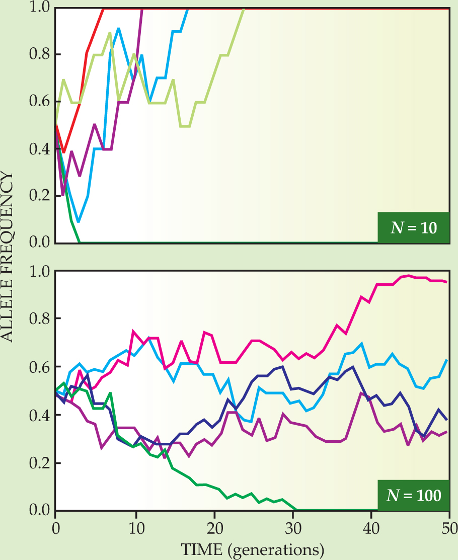
The fluctuations in offspring number cause an initial population with multiple alleles to become genetically uniform after a so-called fixation time on the order of N generations. To good approximation, the stochastic dynamics of the allele frequency can be described by a diffusion process with an f-dependent genetic diffusion constant D of order f(1−f)/N, as discussed in
The states f = 0 and 1 cease to be absorbing when one considers mutations arising at a small nonzero rate µ per generation. The system now approaches a statistically steady state after about N generations, with an average gene frequency 〈f〉 between 0 and 1. If one follows the lineages of two neutral alleles backwards in time, it turns out that they coalesce into their most recent common ancestor after a number of generations that is again of order N.
After they separate, both lineages accumulate mutations at the rate µ, so the expected number of differences is of order 2µN. Genetic diversity caused by rare mutations should increase with population size because genetic variation in larger populations is more slowly eliminated by number fluctuations, which decrease like
How do small advantages in reproductive success alter the prospects of a mutation, and when does that Darwinian selection stand out against a background of neutral evolution? In the simplest model, mutants are assumed to have a factor 1 + s more offspring per generation than nonmutants. (If the mutation is slightly advantageous, s is positive and much less than 1.) Thus the ratio of mutants over nonmutants initially increases exponentially at a rate s. Hence, in the absence of genetic drift, a newly introduced beneficial mutation is expected to take over the whole population after some ln(N)/s generations.
Number fluctuations can, however, dramatically alter that deterministic Darwinian scenario. Many newly appearing beneficial mutations are not, in fact, destined to reach fixation, because genetic drift causes them to hit the f = 0 absorbing boundary first. The relative strength of selection and genetic drift is controlled by the product Ns, which compares the fixation time N with the adaptation time 1/s of the beneficial mutation. For Ns much less than 1, beneficial alleles are effectively neutral and reach fixation with a probability of about 1/N. But even when Ns is much greater than 1, fixation of the beneficial allele is far from certain. It occurs with a probability of only 2s (see
Spatial structure and stepping stones
The above results apply to well-mixed populations whose distribution has no substantive spatial structure. That restriction excludes many cases of interest. In species with nontrivial spatial distributions, any evolutionary novelty first arises in one individual at one location and must then spread across the habitat. And one expects that nearby individuals are more closely related than individuals far apart.
Spatial structure seriously complicates population-genetics models. In a mean-field approximation, spatial migration of alleles can be modeled as an effective mutation rate. Kimura recognized that neither well-mixed (zero-dimensional) nor mean-field (infinite-dimensional) models could explain the genetic diversity that increased with distance between individuals in many species.
1
He and George Weiss constructed a spatial stepping-stone model that consists of a one- or two-dimensional array of discrete islands, called demes (see
In nonequilibrium statistical physics, stepping-stone models with each island housing a single individual are called voter models. 5 Imagine that every deme in a stepping-stone model starts out with a population N greater than one in a mixture of two neutral alleles, A and B. Then genetic drift will tend to locally decrease the diversity of the mixture in favor of one of the alleles. Thus regions of demes emerge that are dominated by either A or B. The size of those domains then increases diffusively as the square root of time. In the absence of mutations or selective advantage, the domain sizes grow without bound, and eventually the entire population becomes either all A or all B.
Under the right conditions, 2D microbial range expansions provide an excellent illustration of the dynamics of 1D stepping-stone models. In the bacterial colony shown in figure 2, a 50–50 mixture of two strains of flagellaless mutant Escherichia coli bacteria has been transferred from the edge of a razor blade onto a line bisecting the surface of a Petri dish whose hard agar nutrient substrate essentially immobilizes them. 6 The two strains, grown in the dark, differ only in the color of their very similar fluorescent proteins. That difference can be regarded as genetically neutral.

Figure 2. Fluorescent image of two equally fit color strains of Escherichia coli bacteria spreading by cell division on two fronts from the razor-edge line along which a well-mixed 50–50 population of the two strains was inoculated onto a surface of hard agar nutrient.
As the population spreads by cell division into unoccupied territory on both sides of the blade line, genetic drift causes the two strains to rapidly segregate into red and green domains. The two population waves advance linearly in time. To good approximation, the bacteria stop dividing or jostling their neighbors once they’re well behind the advancing lines of pioneers at the two frontiers. Thus the colored domains provide a record of the range expansion, and a 1D stepping-stone model can approximate the dynamics at the moving frontiers of active pioneers.
Genetic drift causes the domain boundaries to wander. Eventually, it seems, each front is completely dominated by a single color. That complete segregation contrasts markedly with the persistent finite domains one gets at long times in most 1D equilibrium-statistical-mechanics models. In fact, many species outside the laboratory seem to be more strongly differentiated over large geographic scales than is predicted by the usual 1D and 2D stepping-stone models with large deme populations, even when they’re generalized to include mutations. To reproduce the observed strong differentiations in a steady-state model, one needs very small deme sizes or very large mutation rates. Strong genetic differentiation can also arise from repeated, vigorous migratory expansions. Genetic differences between separated populations can, of course, also reflect differing ecological selection pressures.
Few exact results are known for spatial models that include natural selection as well as genetic drift. As discussed in
Genetic waves and population waves
Here we describe extensions of the well-mixed diffusion model of
where D = m/2 is the spatial diffusivity and g = 1−f. The forward and backward mutation rates µ and v are defined in
Surprisingly little is known about stepping-stone models when selection, genetic drift, and mutations are all present.


When genetic drift and mutation rates are negligible, beneficial alleles sweep across the habitat in a so-called Fisher genetic wave,
7
in sharp contrast to the exponential growth of beneficial alleles in well-mixed populations. The wave train has a sigmoidal shape and advances at velocity
Fisher genetic waves have been created in vitro by John McCaskill and coworkers using fast-replicating RNA molecules. 18
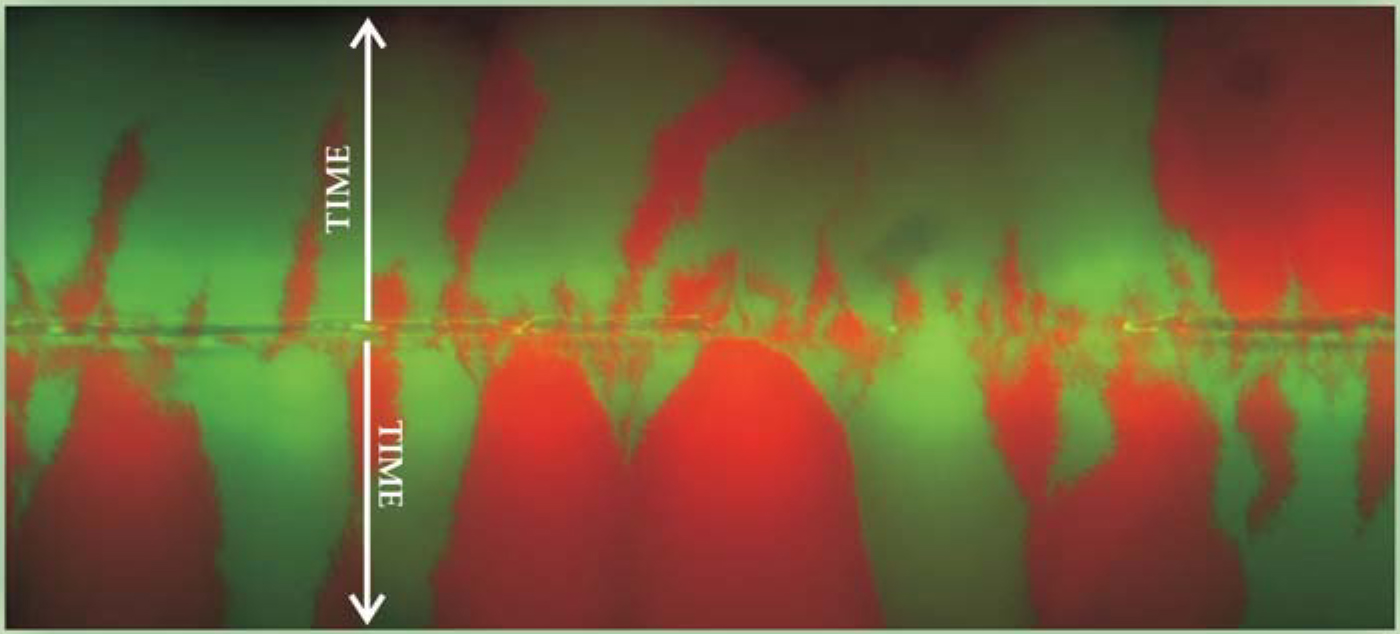
The figure above illustrates a Fisher populafion wave with gene surfing. 14 One sees a radial slice through the 10-cell-thick bacterial colony like those in figure 3 edge-on, thinning at the expanding frontier. Instead of a favorable allele replacing an unfavorable one, two fitness-neutral genetic variants compete at the front of the spreading population wave. In this case, genetic drift not only slows the wave speed but also allows one variant to take over at the front. That’s because each generation of pioneers springs only from parents at the 1D expanding frontier.

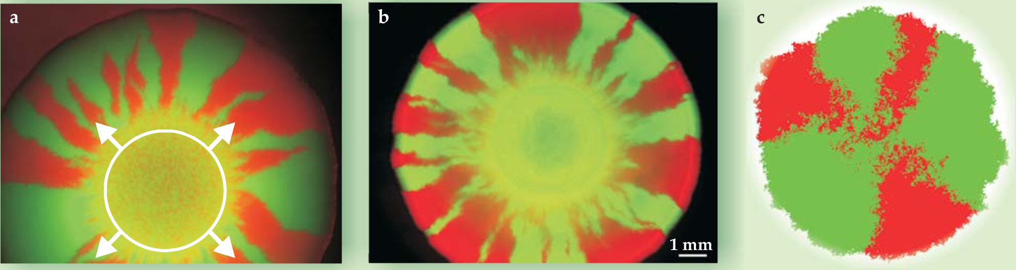
Figure 3. Genetic segregation in radial expansion from a drop of inoculant is demonstrated by microbial colonies of (a) Escherichia coli
((b) figure courtesy of J. Xavier and K. Foster)
Does the neutral theory work?
Whether molecular evolution is mainly neutral or driven by selection has been hotly debated for three decades. Perhaps the most fundamental prediction of the neutral theory is that genetic diversity should increase with population size because genetic variation is less susceptible to elimination by number fluctuations in large populations. One gets a naive test of the neutral theory from nucleotide diversity, a simple measure of a natural population’s genetic diversity. (A nucleotide is just a coding base with molecular adornments that carry no coding information.) For a pair of individuals randomly chosen from the population in question, the nucleotide diversity is just the expected fraction of corresponding DNA sites at which the two individuals will have different nucleotides.
According to both stepping-stone and well-mixed models, the nucleotide diversity thus measured should be linearly related to the product of an “effective” population size N e and the relevant mutation rate. 8 Interestingly, nucleotide diversities are found to differ by less than one order of magnitude across a wide range of species, even though actual population sizes vary over many orders of magnitude. Given that mutation rates (per nucleotide per DNA replication) in multicellular organisms share the same order of magnitude, the similarity of nucleotide diversities means that the N e inferred from the model is often just a tiny fraction of the actual population size. For the much-studied common fruit fly, for example, one infers an impossibly low N e of only about a million for those widely dispersed insects. 9
A number of explanations have been proposed for such small values of N e in species with much larger actual populations. An explanation consistent with the neutral theory is that populations are usually not in a demographic steady state, having varied significantly in size and geographic distribution in their evolutionary past. Consequently, stepping-stone or well-mixed steady-state models may not be appropriate descriptions for their neutral evolutionary dynamics.
Fortunately, there is a test of the neutral theory that largely factors out such demographic uncertainties. It relies on comparing diversities between chromosomes with different abundances in the species population. In humans, for instance, chromosomes come in duplicate pairs except for the sex chromosomes, where the pairing depends on gender. Females carry two X chromosomes, while males carry one X and one Y. Therefore, the population sizes of the X and Y chromosomes are, respectively, 3/4 and 1/4 those of all other human chromosomes. After accounting for the higher mutation rate in male, as opposed to female, meiosis (the cell division that produces the haploid sperm and egg cells), the neutral theory predicts genetic diversities of the X and Y chromosomes that are, respectively, 69% and 31% of the genetic diversity of the other chromosomes. In fact, a study based on 1.4 million single-nucleotide polymorphisms found diversities of 61% for the X chromosome and 20% for the Y chromosome. 10 Much of that variation, it seems, is explained by Kimura’s neutral theory.
An alternative explanation for unusually low levels of genetic diversity is that natural selection has acted very recently—on time scales less than the neutral fixation time. Such a selective sweep reduces genetic diversity because it pushes an entire suite of “hitchhiking” genes—riding along with one that conveys a significant selective advantage—to replace all others at once. In an asexual population, a selective sweep with hitchhiking genes can mimic a population bottleneck—a phase during which an evolving population is temporarily very small.
In sexual reproduction, gene recombination (the transfer of DNA sequences between paired chromosomes during meiosis) mitigates the hitchhiker effect so that only genetic background in the immediate chromosomal vicinity of the beneficial mutation is dragged along as the selective sweep proceeds. The ensuing stochastic process is called genetic draft. It mimics Kimura’s neutral model in many ways, but with a reduced effective population size. 11 Furthermore, genetic draft predicts a negative correlation between genetic diversity and recombination rate. Strong evidence for that anti-correlation is found in the fruit fly, where virtually no diversity is found in the shortest of its four chromosome pairs, which almost never undergoes recombination. The three longer pairs, which do regularly recombine, exhibit much greater genetic diversity. 12 That observation suggests the importance of genetic draft in shaping neutral diversity.
There is currently less evidence for genetic hitchhiking in humans, although intense efforts are under way to detect signatures of ongoing natural selection. Many studies have looked for genetic variants with unusually low levels of genetic diversity as an indicator for recent positive selection. However, given the huge number of gene loci in a genome, low levels of genetic diversity can occur simply by chance. Furthermore, range expansions can easily mimic a selective sweep.
Thus there appear to be only a handful of common gene variants that can be traced unambiguously to natural selection. Perhaps the most prominent case of widespread selection in humans is the persistence into adulthood of lactase production in northern-European populations that evolved during the past 10 000 years. 13 In most other human populations, adults generally lack that milk-metabolizing enzyme.
Radial expansions and inflation
The observed genetic variation in natural populations suggests that demographic or evolutionary disequilibrium might be the rule rather than the exception. Let us discuss in more detail how equilibrium theories fail when populations expand into new territories. Population expansion in space is a recurrent phenomenon in the evolutionary history of many species, ranging from biofilms to humans. Species expand from where they first evolved, invade favorable new habitats, or move in response to environmental changes or, in the case of biofilms, in response to gradients in nutrients, salinity, or ambient temperature.
Such range expansions result in stark differences between the genetic diversity of the ancestral population and those in the newly colonized regions. That’s often because the gene pool for the new habitat has passed through a bottleneck. Genetic demixing stems from the small number of pioneers that happen to arrive in the unexplored territory first. Such essentially random selection of a small gene pool out of a large ancestral one can easily be confused with natural selection for some aspect of fitness. The alteration of the gene pool depends on the specific demographic scenario and encodes precious information about the group’s migration history. 14 Such genetic footprints offer ways to infer, for instance, how humans moved out of Africa 2 or how species respond to climate change. 15
The somewhat artificial range-expansion geometry of figure 2 was relevant to linear 1D stepping-stone models. The radial expansion of neutral bacterial alleles shown in figure 3 emanating from small circular inoculations near the centers of Petri dishes is more relevant to real colonization events by a genetically diverse population of moderate size. For two different types of bacteria, figures
Figure
Unlike the linear inoculation of figure 2, the radial population expansions of figure 3 are subject to inflation: The circular circumference of actively dividing cells at the frontier grows linearly with time, outpacing the diffusive mixing that eventually leads to complete color segregation in the linear-inoculation case. In radial expansion, the “phase separation” predicted by 1D stepping-stone models is incomplete, and the number of distinct sectors remains finite even in the limit of long times.
The striking gene segregation of figure 3, caused in this case by genetic drift, could easily be confused with selection pressures acting locally. In conventional 2D steady-state models without range expansions, such high levels of gene segregation are unexpected. 8 In such models, heterozygosity (the probability that nearby individuals have different alleles) decays rather slowly, like 1/ln(t).
The enhanced gene segregation we find for microorganisms reflects a reduction in dimensionality typical of range expansions. That is, the gene pool for newly colonized regions is sampled from an effectively 1D front population. In the reference frame that moves with the wavefront, the dynamics resembles a 1D population arrayed around a circle. So one gets the faster segregation of alleles expected for a 1D model, with heterozygosity decaying like
The simplicity of the sectoring mechanism suggests that it could be widespread. Indeed, large zones of pronounced genetic homogeneity have been found repeatedly in wild populations of slow-moving organisms such as snails. 14 Such patterns might in fact be explicable in terms of linear or circular range expansions. Because climatic changes have certainly promoted many range expansions, it seems important to take enhanced genetic drift at the frontier (sometimes called gene surfing) into account when interpreting broad phylogeographic trends.
This article has focused on the question of how recurrent population waves alter evolutionary dynamics. The rapidly growing data on genetic variation within and between species challenges our understanding of molecular evolution. Why, for example, are signatures of positive selection so strong in the fruit fly experiments but so weak in human populations? Are patterns of genetic variation more strongly shaped by genetic drift or genetic draft? Another important issue is the effect of the gene proximity on the speed of adaptation in asexual populations. 16 How recombination and interactions between genes shape evolutionary patterns are further important questions. 17 Insights into those central issues of evolutionary genetics should benefit from further developments in genome-wide analyses, modeling, and, hopefully, simple, repeatable experiments on growing microbial populations far from equilibrium.
We acknowledge the support of the Harvard Faculty of Arts and Sciences Center for Systems Biology, as well as comments on our manuscript by Kevin Foster and Pardis Sabeti.
References
1. See J. F. Crow, M. Kimura, An Introduction to Population Genetics Theory, Blackburn Press, Caldwell, NJ (2009).
2. D. L. Hartl, A. G. Clark, Principles of Population Genetics, 4th ed., Sinauer, Sunderland, MA (2007), p. 652.
3. N. A. Rosenberg et al., Science 298, 2381 (2002). https://doi.org/10.1126/science.1078311
4. B. L. Phillips et al., Nature 439, 803 (2006). https://doi.org/10.1038/439803a
5. T. M. Liggett, Interacting Particle Systems, Springer, New York (2005), p. 496.
6. O. Hallatschek et al., Proc. Natl. Acad. Sci. USA 104, 19926 (2007). https://doi.org/10.1073/pnas.0710150104
7. W. Van Saarloos, Phys. Rep. 386, 29 (2003). https://doi.org/10.1016/j.physrep.2003.08.001
8. B. Charlesworth, D. Charlesworth, N. H. Barton, Annu. Rev. Ecol. Evol. Sys. 34, 99 (2003).https://doi.org/10.1146/annurev.ecolsys.34.011802.132359
9. P. Andolfatto M. Przeworski, Genetics 156, 257 (2000).
10. R. Sachidanandam et al., Nature 409, 928 (2001). https://doi.org/10.1038/35057149
11. J. H. Gillespie, Genetics 155, 909 (2000).
12. J. M. Comeron, M. Kreitman, M. Aguadé, Genetics 151, 239 (1999).
13. T. Bersaglieri et al., Am. J. Hum. Genet. 74, 1111 (2004). https://doi.org/10.1086/421051
14. L. Excoffier N. Ray, Trends Ecol. Evol. 23, 347 (2008). https://doi.org/10.1016/j.tree.2008.04.004
15. G. Hewitt, Nature 405, 907 (2000). https://doi.org/10.1038/35016000
16. M. M. Desai, D. S. Fisher, A. W. Murray, Curr. Biol. 17, 385 (2007). https://doi.org/10.1016/j.cub.2007.01.072
17. R. Neher B. Shraiman, Proc. Natl. Acad. Sci. USA 106, 6866 (2009). https://doi.org/10.1073/pnas.0812560106
18. J. S. McCaskill G. Bauer, Proc. Natl. Acad. Sci. USA 90, 4191 (1993). https://doi.org/10.1073/pnas.90.9.4191
More about the authors
Oskar Hallatschek is a physicist at the Max Planck Institute for Dynamics and Self-Organization in Göttingen, Germany. David Nelson is a professor of physics at Harvard University in Cambridge, Massachusetts.
Oskar Hallatschek, 1 Max Planck Institute for Dynamics and Self-Organization, Göttingen, Germany .
David R. Nelson, 2 Harvard University, Cambridge, Massachusetts, US .


