Nonlinear dynamics of heart rhythm disorders

Cardiac arrhythmias are heart-rhythm disorders. Most arrhythmias are not life threatening, and many are benign. But some rhythm disturbances originating in the ventricles—the heart’s main pumping chambers—can be fatal.

Visual observations of animal hearts, documented at least as far back as the 16th century, revealed that the exposed surface of a ventricular wall can break down into worm-like regions or “fibrils” that appear to twitch randomly before death. In an article published in 1874, the French physician and neurologist Edmé Vulpian coined the term mouvement fibrillaire to describe the quivering motion that stops the heart from pumping.

In a human heart, ventricular fibrillation is almost always fatal. It is generally preceded by a very rapid rhythm known as ventricular tachycardia. Roughly half of the deaths caused by cardiovascular disease are sudden. The majority of those sudden deaths—an estimated 300 000 per year in the US—are associated with ventricular fibrillation.

The prevention of sudden cardiac death remains a major clinical challenge. One issue is risk stratification, which entails developing reliable predictors of arrhythmias for different heart diseases. For example, 5 million heart-failure patients in the US are at increased risk of lethal arrhythmias, and roughly 1 in 12 will die within a one-year period. What puts one patient more at risk than another?

The other important issue is therapy. At present, the only effective therapy for treating high-risk patients is an implantable defibrillator that administers a strong electric shock to reset the heart to a normal rhythm. That therapy is invasive and expensive. Moreover, electrical shocks are painful and problematic for patients with frequent arrhythmias. From that standpoint drug therapies are, in principle, preferable if they can be made as effective as implantable devices. But in an arrhythmia-suppression trial conducted in the late 1980s, the death rate was actually higher among patients treated with drugs than among those given placebos. That trial, and several others since, point up the danger of empirical drug therapies. Such problems highlight the urgent need for a better understanding of the genesis of life-threatening arrhythmias and for new therapeutic approaches.

We will use the concrete example of cardiac alternans to illustrate how interdisciplinary research at the intersection of physics, biology, and medicine is helping to fulfill the need for new therapeutic approaches. The study of alternans links basic science to clinical practice. Moreover, it pertains directly to a central question of arrhythmogenesis: How can one foresee an impending lethal arrhythmic event and take steps to prevent it?

Alternans are period-doubling oscillations of electrical or chemical signals in the heart that repeat every two beats. A long history links these signals to sudden death. More generally, period doubling is a well-known hallmark of the onset of chaos in nonlinear dynamics. But that classic route to chaos is not what links alternans to arrhythmias. The relevant signals are arrhythmogenic patterns of asynchrony, in which period-doubling oscillations become spatially out of phase. To understand the arrhythmogenic patterns, researchers must cope with the bewildering biological complexity of the heart, and they must elucidate a wealth of dynamical phenomena that span molecular, cellular, and tissue scales.

Pulsus alternans

Cardiac alternans are abnormalities in which one or more properties of the heartbeat alternate from beat to beat, but the interval between beats is still regular. ¹ Although alternans by themselves are not life threatening, they are often seen in patients with arrhythmias. In 1872, the German physician Ludwig Traube coined the Latin term pulsus alternans to describe a regular heart rhythm with an alternation of strong and weak pulses, as recorded by a beat-to-beat variation of arterial pressure (figure 1a), and he linked this phenomenon to the cardiac death of a patient. With the advent of electrocardiography in the early 20th century, a different facet of alternans was revealed as beat-to-beat variations in the so-called T-wave portion of the electrocardiogram trace (figure 1b).

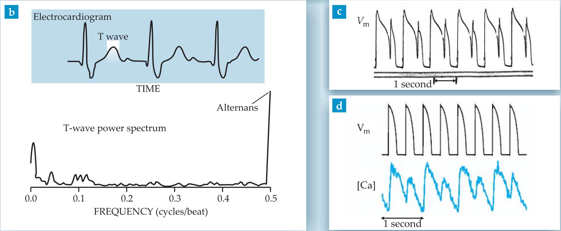
The T wave indicates the electrical repolarization of the ventricles after each contraction. For many decades, reports of T-wave alternans in sudden-death victims remained largely episodic. In the 1990s, however, clinical trials systematically investigated the statistical correlation between T-wave alternans and survival rate for a large number of cardiac patients. ² Those trials established a clear correlation between T-wave alternans and arrhythmia risk.

Nowadays a diagnostic T-wave alternans test is used as a predictor of sudden death. Because T-wave alternans are often too weak to be detected simply by visual inspection of an ECG, the test involves computing a Fourier power spectrum of the T wave (see the lower panel of figure 1b). Such a test is considered positive, meaning that a patient is at increased risk of sudden death, if the peak in the power spectrum at half the heartbeat frequency is sufficiently high above the background noise at other frequencies. This power-spectrum test for alternans received approval from the Food and Drug Administration in 1999, and Medicare announced its coverage just a year ago.

The clinical studies do not explain why T-wave alternans are causally linked to lethal arrhythmias. But major insights have emerged from experiments that explore, with millimeter resolution, the spatiotemporal distribution of cardiac activity on the ventricular surfaces. An individual cardiac cell is about 0.1 mm long and 0.01 mm wide. On that cellular scale, cardiac activity is characterized by two dynamically coupled signals. The first is an electrical excitation that propagates as a wave through heart tissue to make the atria (the heart’s two receptor chambers) and then the ventricles contract. That wave originates from the heart’s natural pacemaker, an area of spontaneously beating cells in the upper region of the right atrium. The change in the voltage difference V _m across the cell membrane associated with that excitation is called the cardiac action potential.

The second signal is chemical. Excitation triggers the release of free Ca²⁺ ions from calcium stores inside each cell. This causes a brief increase of intracellular Ca concentration—the so-called calcium transient. The Ca rise activates the cell to produce a contractile force along its major axis. The total force from a few billion cells produces the cardiac pulse, and the sum of the ion currents from all the cell membranes during the end phase of the action potential produces the T wave in the ECG. Figures 1c and 1d exhibit alternans on the cellular level in traces of V _m and intracellular Ca concentration. ^3,4

Concordant and discordant alternans

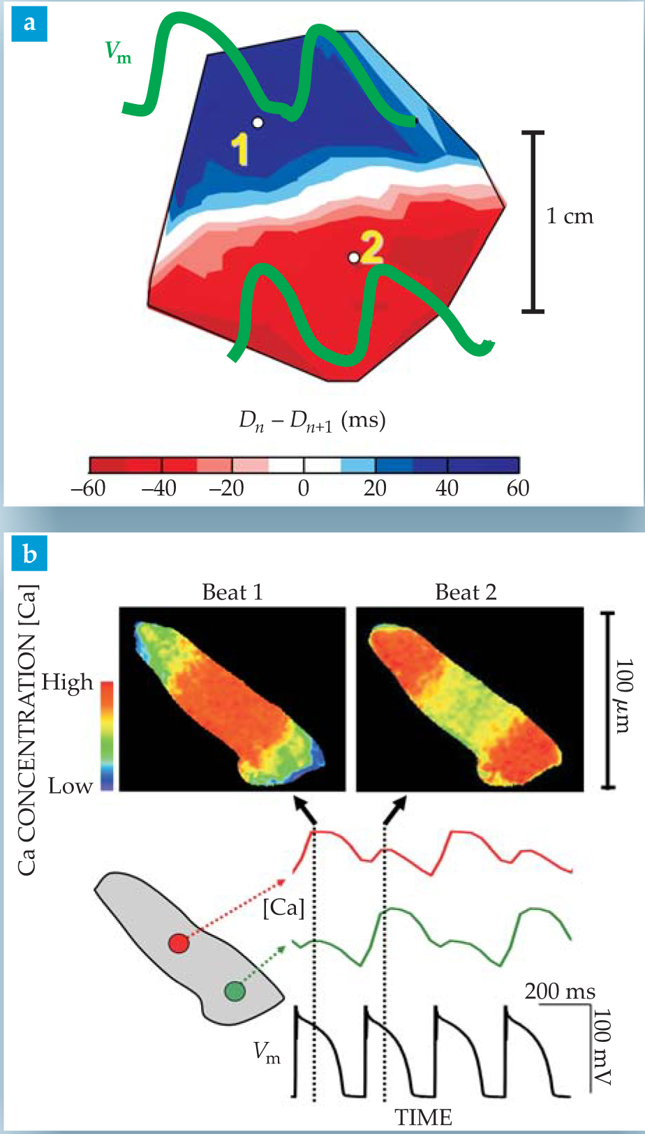
In a 1999 experimental study that causally linked cellular alternans to T-wave alternans, Joseph Pastore and coworkers at Case Western Reserve University used optical mapping to study the spatial distribution of period-doubling oscillations of V _m on the surface of a guinea-pig heart. ⁵ They imaged the electrical activity with a photodiode array that recorded changes in the fluorescence of a dye that binds to the cell membrane and detects the change in membrane voltage.

The group controlled the heart’s rate with an implanted pacemaker electrode. When the heart rate was made fast enough, alternans appeared that were concordant. That is, they were in phase throughout the whole cardiac tissue. With a further increase in heart rate, however, the oscillations became discordant, that is, spatially out of phase in two macroscopic regions of tissue (see figure 2a). And raising the heart rate still further induced fibrillation. Both concordant and discordant alternans produce T-wave alternans in an ECG. But Pastore and coworkers demonstrated that the discordant state is the one that is relevant for the onset of a lethal arrhythmia.

The arrhythmogenic role of discordant alternans stems from the well-established concept that spatial heterogeneity of electrical properties in the heart promotes the onset of lethal arrhythmias. A key property is called “refractoriness.” After being excited, a cell is in a refractory state. That is, it cannot be excited again until after some time interval, the so-called refractory period, which is proportional to the duration of the action potential. One might think of the spread of cardiac excitation as a forest fire. After a fire, an interval is necessary for a new forest to grow before the next fire can spread. Thus the propagation of a forest fire, or a cardiac excitation, fails if the wavefront encounters a region that is still refractory after the passage of a previous wave.

The propagation failure can be local; some islands of trees take longer to regrow than others. Such spatial heterogeneity is known in the cardiology literature as dispersion of refractoriness. Local propagation failure is arrhythmogenic because it produces a wave break that can initiate a pair of counter-rotating spiral waves (see the article by Leon Glass in August 1996, page 40 ). Self-sustained spiral waves are robust patterns that can be seen in a wide range of excitable media. Because colliding waves annihilate in cardiac tissue, high-frequency spiral waves suppress the normal waves emitted by the heart’s pacemaker, and they drive the fast rhythms characteristic of ventricular tachycardia and fibrillation.

Dispersion of refractoriness is present in a normal heart, but it doesn’t suffice to initiate arrhythmias. The traditional view has been that heart diseases facilitate the initiation of arrhythmias by rendering cell properties more heterogeneous. Discordant alternans, however, accentuate or create dispersion of refractoriness “dynamically.” Such dynamic dispersion is due to the alternation of the refractory period from beat to beat, with opposite phases in two regions of tissue. Thus, on any given beat, the refractory period is longer in one region than the other, and vice versa at the next beat. During concordant alternans, by contrast, the refractory period alternates in phase in the whole tissue and thus produces no additional dispersion.

New insights into the genesis of alternans come from recent experiments that probe calcium signaling on a wide range of scales with calcium-sensitive dyes. One remarkable finding is that calcium alternans can become discordant on subcellular scales, as illustrated by the experiments of James Weiss and coworkers at UCLA shown in figure 2b. On a larger scale, Andrew Wasserstrom’s group at Northwestern University has used laser scanning confocal microscopy to image calcium signaling across a dozen cells during alternans in an intact heart. ⁶ The Northwestern work revealed a rich variety of domain patterns: Depending on pacing frequency, the size of synchronized regions of alternans ranged from a fraction of a cell to the whole domain being imaged.

On even larger scales, optical mapping studies of whole tissue cultures have demonstrated the existence of complex spatiotemporal patterns of calcium and contractile activity resulting from the interaction of alternans and spiral waves. ⁷

Calcium transients can affect refractoriness through their effect on membrane current and voltage. But because membrane voltage diffuses much faster than calcium, Ca alternans can influence refractoriness only if they are synchronized over tissue regions greater than a millimeter. Understanding how and when alternan synchronization occurs will require experimenters and theorists to bridge the gap between subcellular and tissue scales.

Symmetry breaking in a heart cable

The existence of the arrhythmogenic patterns of asynchrony in the heart raises a number of fundamental questions. By what mechanisms do those patterns form? How do the mechanisms depend on electrophysiological properties of cardiac tissue and on the frequency of pacing? And from a more practical viewpoint, how can the asynchrony patterns be controlled or suppressed to prevent arrhythmias?

Over the past few years, experiments and computer studies of simple and detailed models of cardiac activity have shed some light on those questions. ^8–11 Nonequilibrium patterns ranging from stripes and hexagons in heated fluid layers (Rayleigh–Bénard convection), to Turing structures in reaction–diffusion systems, to wind-generated sand ripples, are known to form when linear instabilities spontaneously break the translation symmetry of some underlying homogeneous state by amplifying small perturbations. It is now understood that discordant alternans can also result from such a symmetry-breaking instability. The translationally invariant homogeneous cardiac state is the one in which refractoriness is spatially uniform. Spontaneous symmetry breaking produces arrhythmogenic dispersion of refractoriness.

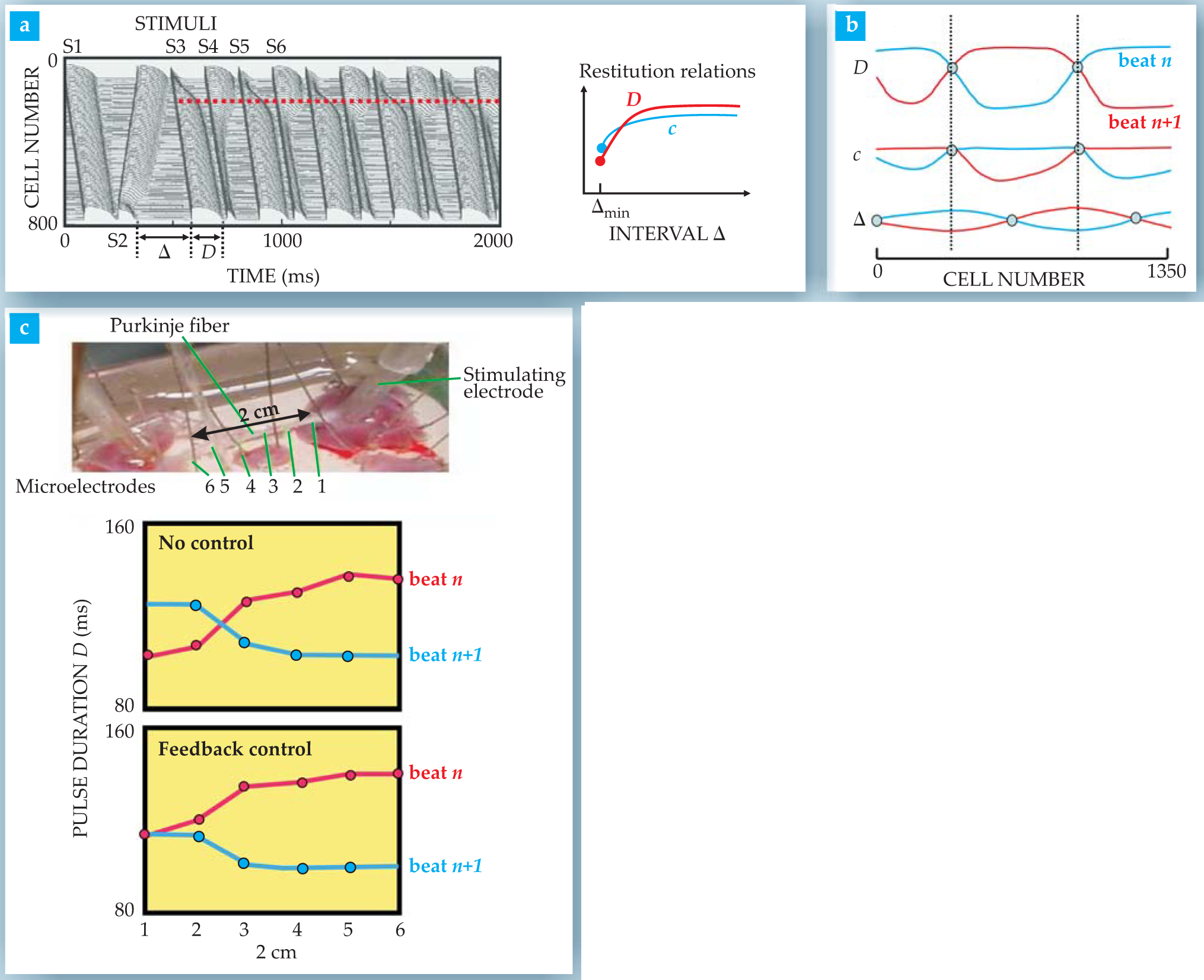
Figure 3 shows computer simulations and experiments that illustrate the formation of nonequilibrium patterns under different pacing protocols in a one-dimensional cable geometry in which all cells are assumed to have identical dynamical properties. The experiments use Purkinje fibers, which are long cable-like strands of heart cells that approximate the idealized computer-model geometry. The computer simulations are based on a Hodgkin–Huxley ionic model for the cardiac action potential (see the box 1 on page 55). Despite their idealized geometry, the computer simulations yield basic insights into the complex arrhythmias of real hearts.

Figures 3a and 3b show the result of a numerical simulation by one of us (Karma) and coworkers for a chain of resistively coupled cells. ⁹ In figure 3a, the discordant alternans are initiated by a so-called ectopic beat. In the pathology of a real heart, an ectopic beat is generally a mistimed pulse originating from a location in the heart different from the heart’s normal pacemaker. Ectopic beats are common, and they can trigger arrhythmias.

The simulation shows the effect of a single ectopic beat on the pattern of membrane voltages as a function of time and position along the cable of cells. The first pacemaker stimulus (S1) applied at the top end of the cable generates a pulse that propagates down the cable at constant velocity. A second stimulus (S2), applied at the cable’s bottom, represents the abnormal ectopic beat. It generates a pulse that propagates up the cable. Subsequent normal pacemaker stimuli at the top end are equally spaced in time. The discordant alternans form suddenly; they begin already with the third beat.

Figure 3b shows the result of a simulation in which the cable is paced at constant period, always from the same end. In that case, it takes several dozen beats for discordant alternans to appear spontaneously. But when they do appear, they form as a periodic pattern of out-of-phase domains with an intrinsic length scale that’s independent of cable length. Our recent experimental realization of this phenomenon with a Purkinje fiber is shown in figure 3c.

Complexity from simplicity

We now turn to the theoretical interpretation of these simulation patterns. A recurring question is, How much of the biological complexity of cardiac electrophysiology should be included in a computer model? Experience has shown that some basic aspects of arrhythmogenesis can be understood by focusing on a few simple empirical laws. That’s not surprising from the perspective of physics, in which complex dynamical phenomena are known to emerge from simple laws.

Directly relevant for understanding the genesis of alternans are the restitution properties of cardiac tissue that we introduced with the forest fire analogy. If the interval after a fire is too short for a forest to be completely regrown, the next fire will be shorter and will not spread as quickly. Similarly, after the end of an excitation pulse, the tissue recovers its resting electrical properties over a finite time interval such that both the pulse’s duration and its velocity depend on the interval between pulses. These dependences are embodied in the restitution curves of figure 3a. A steep curve of action-potential duration versus recovery interval promotes alternans.

That relation was first explained in 1968 by Jesus Nolasco and Roger Dahlen ³ by means of a cobweb-like graphical construction now common in textbooks on nonlinear dynamics. For periodic pacing with period τ, their construction is equivalent to the iteration map

$$D_{n+1}=f\left({\Delta }_n\right)=f\left(\tau -D_n\right)$$ ((1))

that relates the duration D of one action-potential pulse to the one before. The function f is the red restitution curve in figure 3(a).

This iteration map exhibits a period-doubling bifurcation if the slope of f at its so-called fixed point (where further iteration no longer changes D) exceeds unity. The map doesn’t always predict the onset of alternans accurately. That’s probably because it neglects the coupling of voltage to calcium concentration. But it does provide a useful starting point for understanding alternans in tissue.

Let us now interpret discordant alternans from the broader standpoint of symmetry breaking. The phase of period-doubling oscillations is degenerate by π, which means that the pulse-duration sequences long-short-long-short and short-long-short-long are equivalent. This discrete symmetry is identical to the up–down symmetry of the classic Ising model of ferromagnetism. Below the Curie temperature, up and down domains of opposite magnetization have equivalent thermodynamic properties. Therefore a wall between two such domains is stable in one dimension. In the example of figure 3a, symmetry is broken explicitly by the misplaced ectopic stimulus at the cable’s far end, and the resulting discordant alternans formed at subsequent beats are directly analogous to magnetic domain-wall patterns.

But fundamental differences between magnetic patterns and discordant alternans do arise when out-of-phase cardiac domains form a pattern with some intrinsic spatial periodicity, as in the example of figure 3b. In that case, symmetry along the cable is broken by a subtle pattern-forming linear instability that has no magnetic analogue. This instability, which develops over many beats during periodic pacing at one end of the cable, arises because pulse velocity depends on the recovery interval Δ. That generates an effective nonlocal coupling between period doubling oscillations in different regions of the cable.

To see why, let us compute the time interval between the arrival of two consecutive pulses at a position x along a cable that is paced at constant period τ at its x = 0 end. When the velocity c is constant, the time for one pulse to reach x is just x/c. But when the velocity varies spatially, that time becomes an integral of dx/c. Therefore, the difference of arrival times between the pulses at beat n and its predecessor is simply

$$T_n\left(x\right)=\tau +{\int }_0^x\left[\frac{1}{c\left({\Delta }_n\left(x^{‘}\right)\right)}-\frac{1}{c\left({\Delta }_{n-1}\left(x^{‘}\right)\right)}\right]d{x}^{‘},$$ ((2))

where c(Δ) is the functional dependence of conduction velocity on recovery interval shown by the blue curve in figure 3a.

The dynamical consequences of this nonlocal coupling for pattern formation of small-amplitude alternans has been analyzed by one of us (Karma) and Blas Echebarria ¹⁰ in the theoretical framework introduced in the 1950s by Vitaly Ginzburg and Lev Landau in the context of superconductivity and widely used since then to study phase transitions and pattern formation. This analysis, which rests on an analogy between symmetries of magnetization and cardiac period doubling, predicts the existence and scale of standing- and traveling-wave modulations of alternans that have indeed been experimentally observed. Also, the recent extension of that analysis that includes the coupling of intracellular calcium to membrane voltage links the formation of subcellular discordant alternans like those in figure 2b to Turing structures. ¹¹

Control of alternans

Finding means to control alternans is important from a therapeutic standpoint, given their link to arrhythmias. There are, in principle, two routes to that end. One is to suppress alternans with drugs that alter the properties of one or more kinds of ion channels. Drugs that flatten the restitution curve of action-potential duration D versus Δ in figure 3a have been shown to have an antifibrillatory effect in laboratory animals. ¹² But those particular drugs would be lethal in humans. Moreover, if calcium dynamics is the cause of alternans, it is not clear what should be the pharmacological target.

The other approach is to use an implantable electrical device that simultaneously records the electrical activity of the heart and delivers low-amplitude stimuli designed to suppress alternans. ¹³ Several studies have demonstrated its feasibility, but successes to date remain limited to zero-dimensional applications, that is, cases in which alternans are manifested only temporally in small tissue patches. Therefore one has to ask whether such devices can also suppress spatiotemporal patterns such as discordant alternans.

The cardiac cable geometry serves as a good test bed to address that question. ^10,14 In particular, it provides the freedom to record the electrical activity at some control site and then to feed that information back to modify the interval between stimuli delivered by a pacemaker. That task could be assigned to an implantable device in a real heart. Let x _c designate the position of the control site along the cable, and place the pacemaker at the cable’s left end (x = 0). One could, for example, modify the interval between the nth and (n+1)st pacemaker stimuli by an amount proportional to the difference of pulse durations of two consecutive beats at x _c. That is, $$T_n\left(0\right)=\tau +\gamma \left[D_n\left(x_c\right)-D_{n-1}\left(x_c\right)\right],$$ ((3))

where γ is the feedback gain.

The efficacy of this scheme can be addressed through the Ginzburg–Landau theory. ¹⁰ For a short cable in which the pulse velocity is approximately constant, the theory predicts that feedback control simply produces regular standing waves with a single node very close to x _c. Figure 3c illustrates the experimental validation of this prediction with a Purkinje fiber on which the pacing is actually done at the feedback control site. ¹⁴ As predicted, the pattern of discordant alternans is transformed by feedback control into a standing wave whose node coincides with the control site.

Alternans generally start in some localized region of the ventricles. The feedback scheme offers the possibility of suppressing such alternans by recording in the ventricular region while pacing the heart from another region. But alternans can’t be suppressed so easily if they are present in a large region of the ventricles. In figure 3c, for example, the alternans are still present at the antinode of the feedback-controlled standing wave. How the feedback scheme might deal with that problem is an active topic of research.

From cables to real hearts

How can basic insights into alternans obtained in a 1D cable—not even the physicist’s proverbial spherical cow—be used to understand the onset of fibrillation in a real heart? The real heart differs from the cable not only by its three-dimensionality but also by the spatial variation of tissue properties that is an inherent part of its architecture.

For hundreds of millions of beats, these heterogeneities do not disturb the normal pattern—until the sudden onset of a lethal arrhythmia. Are arrhythmias in a real heart due to the same dynamical processes that enhance dispersion of refractoriness in a spatially homogeneous cable? The clinical link of T-wave alternans to sudden death supports, but does not prove, this conjecture.

The results of experiments and computer simulations that link cables to real hearts are shown in figure 4. The work was motivated by the observation that complex sequences of premature ectopic beats often trigger lethal arrhythmias. The link was convincingly established by a theoretical model incorporating measured restitution curves from a real dog heart in a cable simulation to predict which sequences of premature beats are most likely to cause propagation failure. Those lethal sequences were then used to pace the real dog heart and reliably induce fibrillation.

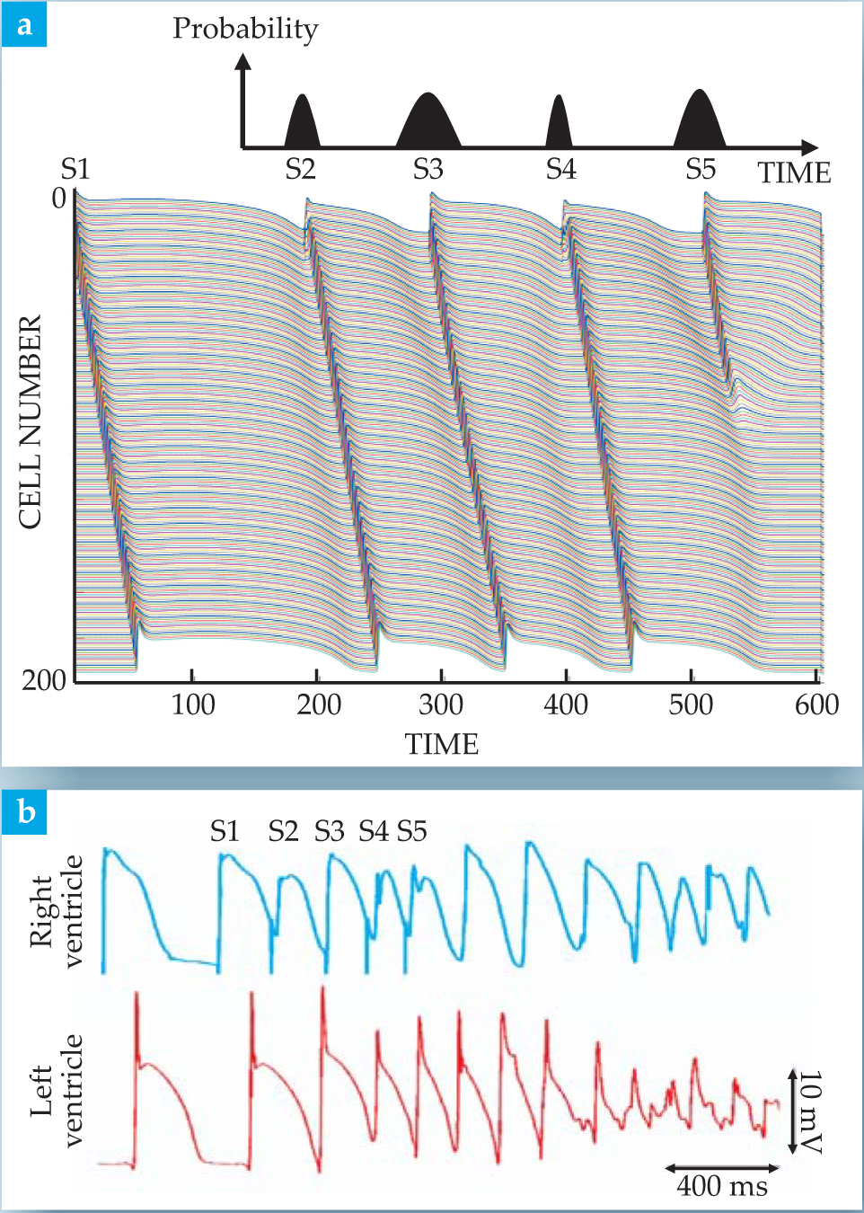
The computer studies, carried out by one of us (Gilmour) and coworkers at Cornell, used the cable equation (see the box 1 on page 55) and a set of spatially coupled iterative maps based on measured restitution curves. ¹⁵ The model extended equation 2 to aperiodic pacing. Figure 4a shows the most lethal aperiodic five-pulse pacing sequence predicted by the model. An initial stimulus at the beginning of the cable, followed by a sequence of four premature successors, produces spatiotemporal variations of pulse duration and refractory period that culminate in the failure of the last pulse to propagate. The failure occurs when the pulse encounters a site along the cable where the interval between two waves falls below the minimum recovery time necessary for propagation. As in the simulation shown in figure 3, dispersion of refractoriness is produced dynamically by restitution kinetics—that is, by the relation between the pacing time sequence and the dependence of pulse duration and velocity on recovery time.

The pacing sequence of figure 4a turned out to be the one most likely to induce simulated fibrillation. It involves alternating short and longer recovery intervals Δ between successive pulses at the beginning of the cable. It is this alternation that drives the cells along the cable at their natural period-doubling frequency, thus amplifying oscillations that would otherwise damp out. The amplification ultimately causes propagation failure when Δ falls below the requisite minimum. The black curves above the four premature stimuli show the relative probability of such propagation failure before the end of the fifth wave when a particular stimulus is shifted slightly from its most lethal time.

How do the simulation results compare with real hearts? Figure 4b shows action-potential recordings obtained from the right and left ventricles of an anesthetized dog during delivery of multiple premature stimuli to the right ventricle. Delivery of the most lethal sequence predicted by the model did indeed induce fibrillation. In eight animal experiments thus far, the model—when it incorporated measured restitution relations—accurately predicted which pacing sequences would produce fibrillation and which would not.

Prospects

The above examples reflect a departure from the traditional view that congenital anatomical heterogeneities in the heart, exacerbated by various diseases, are the main cause of lethal arrhythmias. Arrhythmogenic patterns such as discordant alternans can also arise spontaneously from symmetry-breaking dynamical instabilities in homogeneous tissue. Moreover, these dynamical instabilities can potentially be more lethal than anatomical heterogeneities.

The interaction and relative importance of anatomical and dynamical heterogeneities remain to be explored. There is hope that suppressing dynamical instabilities, either pharmacologically or by low-amplitude stimuli, may prevent arrhythmias in some patients. But it will undoubtedly fail for others, for whom anatomical heterogeneities make fibrillation inevitable.

Relevant for the latter group of patients, research is focused nowadays on elucidating wave processes that come after the onset of a lethal arrhythmia. Considerable progress has been made in characterizing wave turbulence manifested as spiral defect patterns on the surface of the fibrillating heart. ¹⁶ Also, new approaches to defibrillation are being developed. ¹⁷

More than two centuries after Vulpian’s description of the mouvement fibrillaire, however, we still do not know what hides beneath the quivering surface of the fibrillating heart. But new subsurface imaging methods are under active study. They range from light-scattering techniques to ultrasound-guided insertion of nanofabricated electrical probes into the ventricular wall. Until these methods can characterize the 3D geometry of fibrillation with adequate spatial and temporal resolution, its origin will remain a subject of debate and finding alternatives to today’s implantable defibrillators may prove difficult.

In the early 1980s, Arthur Winfree pioneered the mathematical study of scroll waves in excitable media and argued that they may play an important role in ventricular fibrillation. But almost three decades later, the dance of those waves in the heart remains elusive.

References

1. J. N. Weiss et al., Circ. Res. 98, 1244 (2006). https://doi.org/10.1161/01.RES.0000224540.97431.f0
2. D. S. Rosenbaum et al., N. Engl. J. Med. 330, 235 (1994). https://doi.org/10.1056/NEJM199401273300402
3. J. Nolasco, R. Dahlen, J. Appl. Physiol. 25, 191 (1968). https://doi.org/10.1007/BF00697663
4. E. Chudin et al., Biophys. J. 77, 2930 (1999). https://doi.org/10.1016/S0006-3495(99)77126-2
5. J. M. Pastore et al., Circulation 99, 1385 (1999). https://doi.org/10.1161/01.CIR.99.10.1385
6. G. L. Aistrup et al., Circ. Res. 99, E65 (2006). https://doi.org/10.1161/01.RES.0000244087.36230.bf
7. H. Bien, L. Yin, E. Entcheva, Biophys. J. 90, 2628 (2006); https://doi.org/10.1529/biophysj.105.063321
S. M. Hwang, T. Y. Kim, K. J. Lee, Proc. Natl. Acad. Sci. USA 102, 10363 (2005). https://doi.org/10.1073/pnas.05015391028. Z. Qu et al., Circulation 102, 1664 (2000); https://doi.org/10.1161/01.CIR.102.14.1664
J. J. Fox, R. F. Gilmour Jr, E. Bodenschatz, Phys. Rev. Lett. 89, 198101 (2002); https://doi.org/10.1103/PhysRevLett.89.198101
J. J. Fox et al., Circ. Res. 90, 289 (2002); https://doi.org/10.1161/hh0302.104723
H. Hayashi et al., Biophys. J. 92, 448 (2007). https://doi.org/10.1529/biophysj.106.0910099. M. A. Watanabe et al., J. Cardiovasc. Electrophysiol. 12, 196 (2001). https://doi.org/10.1046/j.1540-8167.2001.00196.x
10. B. Echebarria, A. Karma, Phys. Rev. Lett. 88, 208101 (2002); https://doi.org/10.1103/PhysRevLett.88.208101
Chaos 12 , 923 (2002).11. Y. Shiferaw, A. Karma, Proc. Natl. Acad. Sci. USA 103, 5670 (2006). https://doi.org/10.1073/pnas.0511061103
12. A. Garfinkel et al., Proc. Natl. Acad. Sci. USA 97, 6061 (2000); https://doi.org/10.1073/pnas.090492697
M. L. Riccio, M. L. Koller, R. F. Gilmour, Circ. Res. 84, 955 (1999). https://doi.org/10.1161/01.RES.84.8.95513. K. Hall et al., Phys. Rev. Lett. 78, 4518 (1997); https://doi.org/10.1103/PhysRevLett.78.4518
G. M. Hall, D. J. Gauthier, Phys. Rev. Lett. 88, 198102 (2002); https://doi.org/10.1103/PhysRevLett.88.198102
D. J. Christini et al., Proc. Natl. Acad. Sci. USA 98, 5827 (2001). https://doi.org/10.1073/pnas.09155339814. D. J. Christini et al., Phys. Rev. Lett. 96, 104101 (2006). https://doi.org/10.1103/PhysRevLett.96.104101
15. J. J. Fox et al., New J. Phys. 5, 101 (2003). https://doi.org/10.1088/1367-2630/5/1/401
16. F. X. Witkowski et al., Nature 392, 78 (1998); https://doi.org/10.1038/32170
R. A. Gray et al., Nature 392, 75 (1998). See also the talks by S. Luther and E. Bodenschatz available at http://online.itp.ucsb.edu/online/cardiac_m06/ . https://doi.org/10.1038/3216417. C. M. Ripplinger et al., Am. J. Physiol. Heart Circ. Physiol. 291, H184 (2006). https://doi.org/10.1152/ajpheart.01300.2005
18. Y. Rudy, J. R. Silva, Quarterly Rev. Biophys. 39, 57 (2006). https://doi.org/10.1017/S0033583506004227
More about the authors
Alain Karma is a professor in the physics department and director of the Center for Interdisciplinary Research on Complex Systems at Northeastern University in Boston. Robert Gilmour is a professor in the department of biomedical sciences at Cornell University in Ithaca, New York.
Alain Karma, 1 Northeastern University, Boston, US .
Robert F. Gilmour, 2 Cornell University, Ithaca, New York, US .