Multiscale modeling beyond equilibrium
DOI: 10.1063/PT.3.4430
Engineered materials exhibit amazing and useful out-of-equilibrium properties. Some are soft but tough; others can harvest waste heat to produce electricity. Their properties often depend on how the materials are processed; during processing they can exhibit complex flow behavior unlike that of simple fluids. Classical descriptions like the Navier–Stokes equation or Hookean elasticity do not capture the mechanics of such materials. Instead, modeling emergent complex behavior requires simultaneous dynamical descriptions on both macroscopic and microscopic length scales (see the

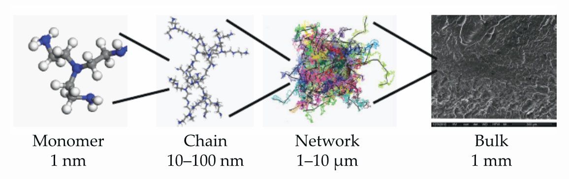
Figure. Polymeric materials exhibit different structures on a wide range of length scales. If a material is deformed, the structures relax on disparate characteristic time scales, from tens of picoseconds for monomers to hours or even years for bulk materials. Models of multiscale materials aim to describe bulk properties by capturing structural dynamics across length and time scales. (Adapted from Y. Li et al., Polymers 5, 751, 2013, doi:10.3390/polym5020751 .)
Complex fluids can exhibit counterintuitive behavior. For example, inserting a rotating rod into a polymer solution or melt will cause the fluid to climb many centimeters up it. Known as the Weissenberg effect, the behavior is opposite that seen in fluids like water, whose flows are dominated by inertia. In simple fluids, a depression in the liquid’s surface forms around the rod. Equally strange, if a bit of polymer liquid is pulled out of the top of a bucket, it can act as a kind of tubeless siphon and continue to flow over the edge on its own accord, as shown in the opening image. (For videos of the effects described here, see reference .)
Solid polymers display many equally interesting phenomena. Because their dynamics slow dramatically as they approach their glass transition temperature—the temperature below which a polymer behaves like a solid but remains noncrystalline—many polymers never reach equilibrium on cooling. In practice, polymers are not always uniform enough to fully crystallize. Solid, fully crystalline polymers are therefore scarce. If solidification occurs by rapid cooling either during or immediately after the material is deformed, the sample will stay deformed as long as it remains below the glass transition temperature, but it will go back to its original shape when heated. Applying a large plastic deformation to a solid polymer causes chain segments to become strongly oriented and can produce filaments with ultrahigh stiffness and strength. Those fibers are then used for many applications, such as cut-resistant gloves and strong, lightweight ropes for use at sea. For a more detailed description of semicrystalline polymers, see box
Semicrystalline polymers
Cooling a polymer below its crystallization temperature typically does not result in a fully crystalline material. Instead, crystallization is arrested by topological constraints and a dramatic slowing as the system approaches its glass transition temperature. 12 , 13 Processing conditions, such as how the polymer is cooled and deformed, have a strong effect on the resulting microstructure and determine properties like the volume fraction of crystals, the thickness of lamellae, and the structure’s overall anisotropy.

The diagram outlines how flow-induced crystallization in a polymer can control the material’s mechanical properties. When isotropic polymers (top) undergo a macroscopic deformation, they can become oriented and stretched (right). At sufficiently low temperatures, that stretching enhances their crystallization (bottom). Chain segments locally pack into small organized structures, such as lamellae or shish kebabs, that can assemble into superstructures.
The semicrystalline morphology of those superstructures (left) can affect the macroscopic behavior of the crystallizing material, including its effective linear elastic properties, yield stress, birefringence, and conductivity. When producing ultrahigh-strength polymer fibers, crystallinity is relevant only during the intermediate processing steps. Achieving the desired mechanical properties requires finding the right density of chain entanglements. A lower entanglement density, which can be achieved by dilution, not only helps to produce thin fibers but also increases the fiber’s drawability, which gives the filament its ultrahigh strength. (Image courtesy of Markus Hütter.)
Cross-linked networks of hydrophilic polymers in water form hydrogels that exhibit elastic behavior. Despite being mostly water, double-network hydrogels can sustain very high stresses—up to tens of megapascals—without breaking. Evidence suggests that the gel dissipates energy by irreversibly breaking the covalent bonds of one network while maintaining its strength through the second, unbroken network.
Simple beginnings for complex behavior
Continuum mechanics provides a well-established foundation for describing the macroscopic behaviors of both fluids and solids. Applying momentum conservation to a continuum generates the equation of motion known as the Cauchy momentum equation:
2
Adding a restrictive assumption—that the pressure tensor has the usual isotropic thermodynamic pressure plus a contribution that is linearly proportional to the instantaneous velocity gradient—yields the famous Navier–Stokes equation. The assumption implies that deformations on molecular length scales relax so quickly that the microscopic components of the material always behave as if they are locally at equilibrium. 3 It also guarantees nonnegative entropy production. The idea is intuitively appealing, and for fluids like water, whose small molecules relax rapidly compared with macroscopic strain rates, the Navier–Stokes equation indeed appears to be exact.
However, for polymers, proteins, colloids, liquid crystals, emulsions, and other materials with larger constituent parts, microscopic relaxation rates can become comparable to macroscopic strain rates, which causes the local equilibrium assumption to fail. (See the article by Byron Bird and Charles Curtiss, Physics Today, January 1984, page 36 .) Researchers recognized the shortcomings of the Navier–Stokes equation for such materials early on; they then began searching for a fix, and the field of rheology was born. Although Cauchy’s equation was safe, it contained that unknown pressure tensor term
Like fluid mechanics, solid mechanics also begins with the conservation of linear momentum. However, the resulting equation is usually recast in terms of the Lagrangian deformation field
The simplified fluid description has dissipation with no elasticity; the simplified solid has elasticity but no dissipation. The former implies an infinitely fast relaxation of the material’s microscopic components, whereas the latter implies no relaxation at all. Irrespective of whether one takes a fluid or a solid as the starting point, extension, or rather enrichment, is clearly required to account for the finite-time relaxation found in real materials.
Microstructure
To describe complex solids and liquids, researchers first had to develop the idea of microstructure, which is captured by variables on an intermediate length scale that relax slowly and have a clear connection to a system’s dynamics on the atomistic scale. The number of such variables should be many orders of magnitude smaller than the number of atoms in the system but still capture the physical phenomena of interest. Any discarded degrees of freedom are typically assumed to be near equilibrium and provide a sort of thermal bath for the more slowly relaxing degrees of freedom.
Physical insight from experiments or atomistic simulations can guide the development of evolution equations for microstructural variables. That process, known as coarse graining, 4 raises three questions:
• What are useful microstructural variables?
• What equations describe their evolution?
• How are macroscopic quantities, such as stress, related to the microstructural variables?
Answering each question requires insight, intuition, and innovation. Systematic ways of finding the right microstructural variables rarely exist. But whether the starting point is a fluid or a solid, the goal of incorporating microstructural variables is to bring finite-time relaxation processes into the overall description. Boxes
Crystalline metals
Solid metals are typically imperfect crystals. When they experience sufficiently high stress, new dislocations—line defects in the crystal structure—are created in large numbers. The dislocations cause irreversible plastic deformation by moving through the crystal lattice, 14 , 15 a feature that is absent in the solid mechanics of elasticity. Interactions between dislocations increase the stress required for yielding and result in work hardening. Dislocations can be described in various levels of detail: parametrization of each dislocation, a statistical description of the orientation of dislocation segments, or simply a density of dislocation segments.

The diagram shows different microstructural levels of description for a crystalline metal. A full-detail atomistic lattice with line defects is shown in the lower left. In the lower right is a phase-field description of dislocations that does not explicitly account for the lattice. The upper right shows a large number of dislocations, each of which is represented by a discrete line.
Macroscopic samples are typically not single crystalline. Rather, they are polycrystalline and contain grains—smaller single-crystalline volumes that make up the larger structure seen in the upper left. The presence of grain boundaries hinders the stress-activated motion of dislocations, so the grain size has a strong effect on the plastic deformation behavior of metals; smaller grains make the metal stronger.
Quantifying the rich microstructure and capturing the interplay between the microstructure and the macroscopic behavior depend on exactly which phenomena one wants to study. Macroscopic stress leads to the creation and motion of dislocations, which also couple back to the macroscopic scale. The characteristics of the dislocations, such as their Burgers vectors, density, and velocities, inform the so-called plastic strain-rate tensor on the macroscopic level, which is the key ingredient for enriching elasticity theory with plasticity. (Image courtesy of Markus Hütter.)
More polymer models
Polymers come in multiple shapes and sizes, and different models are needed to describe their dynamics. One example is a simple model for an idealized branched, entangled chain architecture called the pom-pom.
16
Each chain has a linear backbone with

The pom-pom model complies with thermodynamics, and researchers have identified an expression for its free energy that captures both the driving force of the dynamics and the dependence of the pressure tensor on microstructural conformations. The appropriate orientational relaxation is determined by
Solving the pom-pom model requires calculating the velocity field
Similarly, the microscopic dynamics of an ensemble of independent stochastic trajectories can be solved numerically, akin to using Brownian dynamics simulations to extract information from Fokker–Planck equations. A method called smoothed particle hydrodynamics can be used for the macroscopic-level calculations. Embedded in each particle is an ensemble of several thousand coarse-grained polymer chains. The chains are stochastically independent, but all feel the same local velocity gradient. Taking the proper average over the ensemble of chains yields the local polymeric contribution to stress and the self-consistent motion of the particles.
The slip-link model, illustrated here in tandem with smoothed particle hydrodynamics, is used to describe linear entangled chains. It has fewer adjustable parameters and greater fidelity with experiments than the pom-pom model. On the left, an atomistic simulation shows dense polymer chains at equilibrium. Topological analysis can uncover entanglements in each chain, as shown in the next image. Entanglement parameters are found by matching the statistics from all the chains with the coarse-grained slip-link model (center). An ensemble of chains is placed in each particle of the smoothed particle hydrodynamics simulation, shown in the next image, to find the macroscopic flow. Those simulations can then predict the stresses or other macroscopic properties anywhere inside the flow (right). (Image adapted from Mol. Syst. Des. Eng. 1, 6, 2016.)
A concrete set of variables that accurately describes the microstructure in a complex material is paramount. The variables must include sufficient detail about the microstructure, and simplifications must discard only unnecessary information. The model is then more likely to retain the necessary physics to capture many phenomena. For example, a set of microstructural variables might simultaneously describe mechanical and dielectric phenomena, birefringence, and direct structural information obtained by scattering experiments. However, the variables should only retain the necessary physics for the problem of interest. An overly detailed model can become cumbersome and have too many adjustable parameters.
If a wide separation exists between the macroscopic and microstructural length scales, it should be reflected in the variable choice. Typically, a separation of time scales accompanies the separation of length scales, which makes possible the use of fluctuation–dissipation theorems. 5
Without a more prescriptive set of instructions, choosing the variables for each physical system falls largely to physical insight. But that is not a shortcoming. It is an essential step toward physics-based, rather than algorithm-based, coarse graining.
Introducing microstructural variables into a dynamic model should decrease, not increase, the model’s complexity. It should allow observed phenomena to be expressed in physically intuitive terms and relate seemingly distinct aspects, such as how the concept of entangled polymer chains helps elucidate the counterintuitive Weissenberg and tubeless-siphon effects.
Thermodynamics, but with friction
Modeling the nonequilibrium thermodynamics of dynamic, multiscale systems relies on thermodynamic potentials, such as the Helmholtz free energy. The potentials for such systems, which can be derived from statistical mechanics, do not just determine static properties, but also provide the driving forces for the fluxes and relaxation processes of the microstructural variables. Statistical mechanics can also be applied outside equilibrium, not just to macroscopic variables like volume but also to microstructural variables. That strategy was first used by Werner Kuhn in 1934 to describe polymers. 6 However, because the microscopic and macroscopic descriptions have different amounts of entropy, it is important that the free energies on both levels be compatible: Performing two successive coarse-graining steps, from atomistic to mesoscopic and then to macroscopic, must yield the same free energy as that obtained in a single step from atomistic to macroscopic.
Thermodynamic potentials also help to determine with minimal phenomenology the elusive pressure tensor
Once the microstructural variables are chosen, they need associated evolution equations, which must conform to fundamental physical constraints like the first and second laws of thermodynamics and the fluctuation–dissipation theorem. Parameter values for those equations, such as friction coefficients, may have to be obtained from molecular dynamics simulations or another highly detailed description. In practice, that might mean that the system’s dynamics are described on three levels: atomistic, microstructural, and continuum. However, once the necessary parameter values are found, the atomistic simulations can be discarded, and the model is left with only two remaining variable sets: microscopic—or more accurately, mesoscopic—and macroscopic. In simulations, the two sets must communicate with one another at all times.
No monologues, but a dialogue
Multiscale modeling links the dynamics of the structure on the mesoscopic level with a macroscopic dynamic formulation. The time evolution of macroscopic variables like those typically used in fluid and solid mechanics is refined by time-dependent information from the microstructure. The coupling should be bidirectional: A macroscopic deformation distorts the microstructure, and, in turn, the forces of the deformed microstructure give rise to out-of-equilibrium stresses on the macroscale. The pressure tensor is thus not expressed directly in terms of a macroscopic velocity or displacement gradient; rather, it depends on the mesoscale’s structural state. Such a scenario is typical, and nonequilibrium thermodynamics is often employed to achieve bidirectional coupling in a way that is compatible with fundamental principles of thermodynamics. 4
Although derivatives of thermodynamic potentials act as driving forces for dynamics, frictional transport coefficients are also needed to describe relaxation phenomena. Like entropy, friction increases when moving to coarser levels of description. The most famous assertion of that fact is the fluctuation–dissipation theorem, which relates the magnitude of certain fluctuations on one level of description, like forces or velocities, to friction on a coarser level. Originally, the theorem was derived from purely deterministic dynamics without any friction to put restrictions on coarse-grained dynamics.
Models are more useful when they are well-defined mathematical objects and not just computer algorithms. A mathematical object can be tested rigorously for adherence to the principles of thermodynamics. And when an asymptotic solution to a model exists, it can also be used to test the convergence of algorithms. In our own work, we used the mathematical formulation of the slip-link model to derive an algorithm for graphical processors. It exploits the parallel computing power of inexpensive video cards to perform simulations that are two orders of magnitude faster than those on central processing units but that yield identical results. The speedup could not have been achieved without a well-defined mathematical object.
Using a nonequilibrium thermodynamics route for the model formulation guarantees that the first and second laws, among other restrictions, are respected. The numerical algorithm must therefore converge to a thermodynamically acceptable solution. Moreover, forcing the discretized dynamics of the algorithm to obey thermodynamics can improve the numerical stability of the simulations. 7
Everything flows, including microstructure
The quintessential system for applying multiscale modeling is polymers. The simplest microstructural variable for a polymeric liquid, and one that is slowest to relax, is the conformation tensor
Observations of atomistic simulations or the scattering properties of real systems can be incorporated into a conformation tensor. Hence that microstructural variable easily connects simple molecular descriptions to macroscopic phenomena.
But things aren’t always that straightforward: Chain uncrossability in concentrated polymers leads to entanglements. 8 The spacing between entanglements is a length scale that is independent of molecular weight and is intermediate to the polymer’s persistence length and the overall size of the polymer coil. In several articles in the 1970s Masao Doi and Sam Edwards proposed describing the microstructure of a polymer in terms of the probability density for the orientation of a tube segment that surrounds a particular length of polymer. With that level of description and a simple proposal for anisotropic dynamics, their tube model accurately described the stress relaxation in nonlinear step-strain experiments. (For more on polymer entanglement, see the article by Tom McLeish, Physics Today, August 2008, page 40 .)
The single-segment theory of Doi and Edwards is not sufficient to make quantitative predictions or describe more detailed phenomena. That shortcoming led to the development of more detailed models, such as the so-called slip-link models,
9
which have successfully described entangled polymer melts. Their microstructural variables include fluctuations in entanglement number, entanglement spacing, and monomer density between entanglements. The entanglement parameters characterizing the relevant statistics can all be found with atomistic simulations. Because of their finer level of description, the slip-link models discussed in box
No time to relax yet
Plenty of opportunities exist to build new multiscale models. For example, the dynamics that underlie dislocation-based plasticity may not exhibit a clear separation of time scales, 10 which implies that the fluctuation–dissipation theorem might not hold. Systems without time-scale separation clearly warrant further investigation.
Brittle fracture is also governed by communication between large and small length scales, which makes it a good candidate for multiscale modeling. However, unlike the examples above, in which the microstructure exists throughout the continuum and its effects can be averaged, fracture contains an isolated crack tip in an otherwise elastic continuum. The stress field around the crack tip is long ranged and drives the fracture, but the crack tip itself exists on a small scale. Continuum mechanics are therefore typically applied far away from the crack tip, but atomistic and even quantum mechanical descriptions are used nearby. Intricate coupling is needed to connect the two regions. Because it incorporates the effects of disparities in both length and time scales, multiscale modeling offers opportunities for advancing models of brittle fracture.
Although this article focuses on the responses of materials to deformation, similar issues arise when materials are exposed to other stimuli, such as temperature gradients and electromagnetic fields. In those cases, the details of a dynamic multiscale model—the particular choice of variables and the model’s formulation—depend on which stimuli and phenomena are being studied. But the general philosophy of multiscale modeling presented here can still be applied. Multicomponent materials and the coarse graining of active matter, such as molecular motors in a gel or swarms of swimming Janus particles, also present unique challenges that might benefit from multiscale modeling.
Researchers should not think of microstructural variables only as necessary mathematical simplifications. When coarse graining is successful, it yields deep insights into the physics that underlies interesting phenomena and helps scientists develop intuition for molecular engineering. Atomistic simulations are most useful when they are accompanied by a guiding coarse-grained level of description that can facilitate the extraction of useful information. Even when coarse graining fails, it uncovers information about the assumptions that went into it. A coarse-grained model that eliminates some essential physics will fail to agree with experiment, and that in itself is useful to know. So instead of making apologies for coarse graining, we say that one has no excuse for not doing it. 11
Many open questions, both fundamental and practical, remain, and each new problem requires deep physical insight and creative intuition to find the appropriate level of description. Despite their impressive accomplishments, machine-learning algorithms are not likely to uncover the proper way to model entanglements. Physicists have a lot to contribute in the field.
Great progress has been made in developing robust numerical algorithms for multiscale modeling, but it seems that every new model presents unforeseen numerical challenges. Both fundamental and applied mathematicians can make important contributions on that front, and the tools they develop for modeling multiscale systems are not only intriguing from a fundamental perspective. They have tremendous potential for applications in engineering and may eventually lead to the designing of molecules that exhibit desired nonequilibrium properties.

CYNTHIA CUMMINGS

Markus Hütter would like to acknowledge stimulating discussions with Marc Geers, Varvara Kouznetsova, and Theo Tervoort. Jay Schieber would like to thank David Venerus for useful feedback on the manuscript.
References
1. See, for example, the Weissenberg effect, www.youtube.com/watch?v=0-WmJy9edlA ;
the tubeless siphon, www.youtube.com/watch?v=g4od-h7VoRk ;
and recovery on reheating, www.youtube.com/watch?v=3wKNAPJ-0ug .2. R. B. Bird, W. E. Stewart, E. N. Lightfoot, Transport Phenomena, 2nd ed., Wiley (2002).
3. S. R. de Groot, P. Mazur, Non-equilibrium Thermodynamics, Dover (1984).
4. H. C. Öttinger, Beyond Equilibrium Thermodynamics, Wiley-Interscience (2005).
5. R. Kubo, M. Toda, N. Hashitsume, Statistical Physics II: Nonequilibrium Statistical Mechanics, Springer (1985).
6. W. Kuhn, Kolloid-Z. 68, 2 (1934). https://doi.org/10.1007/BF01451681
7. C. P. Zinner, H. C. Öttinger, J. Non-equilib. Thermodyn. 44, 43 (2019). https://doi.org/10.1515/jnet-2018-0038
8. S. F. Edwards, Proc. Phys. Soc. 92, 9 (1967). https://doi.org/10.1088/0370-1328/92/1/303
9. H. Feng et al., Mol. Syst. Des. Eng. 1, 99 (2016); https://doi.org/10.1039/C5ME00009B
J. D. Schieber, M. Andreev, Annu. Rev. Chem. Biomol. Eng. 5, 367 (2014). https://doi.org/10.1146/annurev-chembioeng-060713-04025210. M. Kooiman, M. Hütter, M. G. D. Geers, J. Mech. Phys. Solids 90, 77 (2016). https://doi.org/10.1016/j.jmps.2016.02.030
11. H. C. Öttinger, J. Rheol. 53, 1285 (2009). https://doi.org/10.1122/1.3238480
12. H. E. H. Meijer, ed., Processing of Polymers, Wiley (1997).
13. G. Reiter, G. R. Strobl, eds., Progress in Understanding of Polymer Crystallization, Springer (2007).
14. J. P. Hirth, J. Lothe, Theory of Dislocations, 2nd ed., Wiley (1982).
15. D. Raabe, Computational Materials Science: The Simulation of Materials, Microstructures and Properties, Wiley (1998).
16. H. C. Öttinger, Rheol. Acta 40, 317 (2001); https://doi.org/10.1007/s003970000159
T. C. B. McLeish, R. G. Larson, J. Rheol. 42, 81 (1998); https://doi.org/10.1122/1.550933
W. M. H. Verbeeten, G. W. M. Peters, F. P. T. Baaijens, J. Non-Newtonian Fluid Mech. 108, 301 (2002). https://doi.org/10.1016/S0377-0257(02)00136-2
More about the authors
Jay Schieber is a professor of physics, chemical engineering, and applied mathematics and the director of the Center for Molecular Study of Condensed Soft Matter at the Illinois Institute of Technology in Chicago. Markus Hütter is an associate professor of multiscale analysis of polymer systems in the polymer technology group of the mechanical engineering department at the Eindhoven University of Technology in the Netherlands.


