MemComputing: When memory becomes a computing tool

In that 1997 book, David Deutsch has a fascinating perspective. ¹ It’s one that I share, and it goes against the prevailing understanding of most computer scientists, mathematicians, and pretty much anyone who has even a minimal background in the theory of computation. For them, computation was defined more than 80 years ago by Alan Turing. ² The edifice researchers have built on it—which has led, among other things, to our modern computers—is quite impressive. Those researchers would tell you that the only physics necessary in the field of computation is the one that makes Turing’s ideas practical. That is, physics is just a tool to realize in practice the mathematical concept that Turing envisioned: With better transistors, engineers can make our modern computers faster, more energy efficient, and smaller.

What if instead we take Deutsch’s viewpoint more seriously? In that case, what physics should we use to compute? Deutsch most likely would say quantum mechanics! He was, after all, one of the first proponents of quantum computers. And despite serious roadblocks, they are frequently hailed as the future of computation. ³ But can we go even further and understand computation as more than a mere physical process? Indeed, can we interpret any physical process as some type of computation?

The equivalence of information and computation

To answer that question, consider a pinball machine (figure 1). As a ball is dropped from the top of the machine, gravity drives it toward the bottom. Along the way, the ball scatters off bumpers and, provided it doesn’t get stuck, exits at the bottom. It has no other choice!

Figure 1.

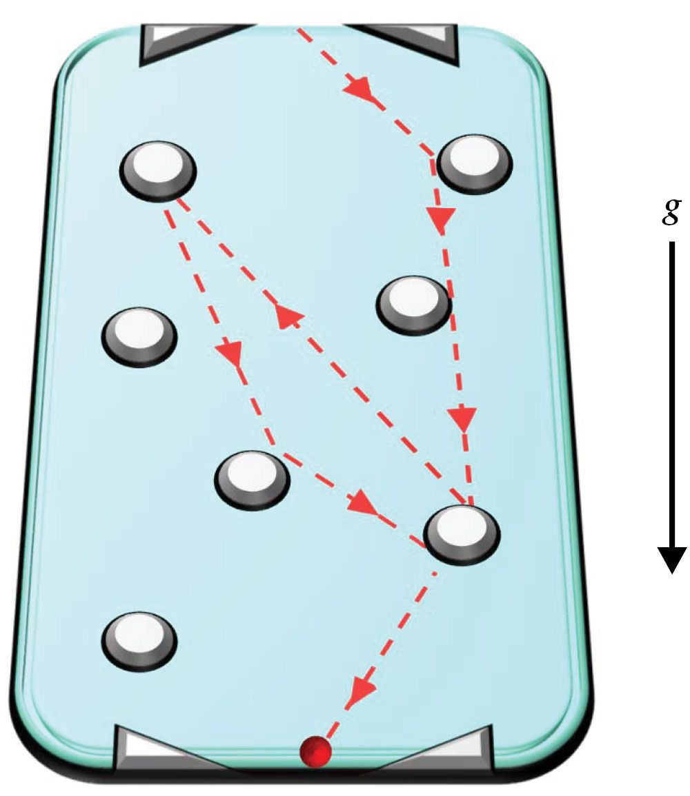
The question is, Can you compute the path the ball follows from the top entrance to the bottom exit? Because I used the word “compute,” you might think of using Newtonian mechanics to calculate the path that an ideal pointlike ball, starting from a given position and velocity, would take while scattering elastically off rigid disks along the walls. You might then turn to modern computers to numerically integrate the equations of motion of the system. And there you have it: You have calculated the ball’s trajectory.

But was it necessary to use modern computers to answer the question? Why not just observe the ball’s trajectory by putting fresh paint on the machine’s surface? After all, the information you want to extract is its trajectory. It does not matter whether that comes directly from the physical system, the ball in the pinball machine, or traditional computation. The actual physical system can calculate its own trajectory infinitely better than the approximate equations used to describe the trajectory. The system includes all possible effects, and the ball doesn’t know or care if such a calculation is difficult. It simply acts according to natural laws. In the process, you would interpret the result as a path or a trajectory.

Indeed, any physical system performs some type of computation, with the observers providing meaning to it. I call that process the equivalence principle between physical information and computation. ⁴ We apply that principle in countless instances without even realizing it—when a thermostat computes the temperature of a room, say, or a speedometer computes a car’s relative speed.

Analog versus digital

You might think that what I have just described is an analog machine—one that, like the temperature on a thermometer or the position of a pinball, operates with real numbers. And analog machines are not efficient at solving combinatorial-optimization problems, such as factoring numbers into their constituent primes. That’s because analog machines are not easily scalable. If you wanted to linearly increase their size—and, correspondingly, the size of the problem to solve—you would need to increase your resources, such as time, space, or energy, exponentially. Because analog machines are sensitive to noise, one would need a digital machine, which maps one finite string of zeros and ones into another finite string of zeros and ones, to solve a combinatorial-optimization problem.

Modern computers operate in real time and manipulate currents and voltages of actual physical devices, such as transistors, with the unavoidable noise and imperfections they carry. Those devices cannot represent mathematical symbols, such as zero and one, with absolute precision. Yet no one would argue that our modern computers are analog machines and hence not scalable. In fact, many scientists believe they are best described as Turing machines, though that is not exactly accurate.

What really distinguishes an analog machine from a digital one is our ability to write the input and read the output of the computation with finite precision—that is, with a finite number of bits. That’s what Turing had in mind, and it’s how our modern computers work. Even though a single transistor cannot exactly represent the mathematical zero (with a low current, say) or one (with a high current), it can represent those values to within an error, or current threshold, that is independent of the size of the machine or the problem to solve. What happens between the input and the output—the so-called transition function in computer-science jargon—is not important for the scalability of the machine, provided the map does not destroy the output of the computation if it is subject to noise or perturbations.

The need for a collective approach

The choice of what physical phenomena should be used to represent the transition function between input and output must be dictated by the goal. If the goal is to solve combinatorial-optimization problems, such as prime factorization, you need to first understand why they can be difficult.

Take, for instance, the Boolean formula in figure 2. It consists of three variables, v₁, v₂, and v₃, related to each other by a logical OR, thus forming a clause, and three different clauses related by logical ANDs. Those variables can take the Boolean values of zero or one. If you ask what logical assignment I need for v₁, v₂, and v₃ to satisfy such a formula—that is, when all the clauses are logically satisfied—then I could randomly assign an initial value to the three variables and sequentially check whether each clause is satisfied.

Figure 2.

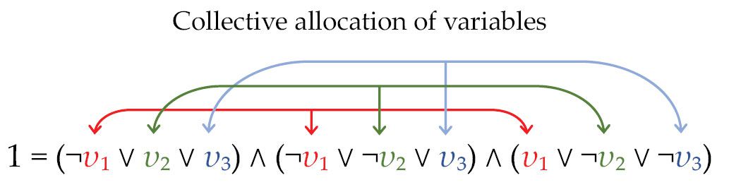
If any are not satisfied, I could change the value of v₁, say, and try again until I find a combination for v₁, v₂, and v₃ that works. That’s easy to do if the number of variables and clauses is just three. But if the number grows to thousands or even millions, as it can in many real-life problems, that approach is not efficient. One may come up with clever algorithms to speed up the process, but for some problems even that approach struggles: The computation time increases exponentially when the size of the problem increases linearly.

The reason for that scaling is that all algorithms are perturbative approaches to computation. They change the value of one or more variables in the problem in a sequential way. Ideally, one would have a machine that assigns the values of a large number of variables collectively, all at once. That collective behavior is nonperturbative. As such, it is reminiscent of strongly coupled systems. And because the machine has to act on a collective number of variables at once in a correlated way, it should have some type of long-range order.

That behavior is typical of continuous phase transitions. Indeed, in the 1990s the theorist Chris Langton suggested that “computation at the edge of chaos”—in the proximity of a critical state of the phase transition—is the optimal condition for processing and storing information. ⁵ But it’s not at all obvious how to practically build a machine that operates at such a sweet spot. In addition, although long-range order is a feature of continuous phase transitions, it may emerge even without a phase transition.

MemComputing paradigm

How can a system self-tune into such a long-range ordered state during computation? The key to that process is memory. By memory, however, I don’t mean storage, but rather time nonlocality—the ability of a physical system to remember its past dynamics in order to perform necessary tasks. I call that computing paradigm MemComputing. ⁶

Time nonlocality may induce spatial nonlocality and drive the system into a long-range ordered state. ³ The process can be intuitively understood with a story. If, for example, I leave pebbles on a trail—forming a “memory trace”—someone else can retrace my path, even if I’ve never met that person and so long as the memory is not somehow displaced. Thanks to that memory trace I can now interact with that person at long distances in a correlated way.

How does that work in practice? Suppose you want to solve a combinatorial problem like the one outlined in figure 2. The idea is to transform the logic gates of the problem into physical systems, such as electronic or optical circuits with specific properties, and then put them together into a single unit. For instance, take the logical OR gate, shown in figure 3. It has only four possible logically consistent states. Then transform the logical variables into continuous ones, which could be the voltages or currents of an actual physical circuit. ⁷ As with transistors, you could set a threshold to some voltage that identifies a logical zero or one, irrespective of how many units you put together. You would then have a digital MemComputing machine, a subclass of the much more general concept of MemComputing. ⁸

Figure 3.

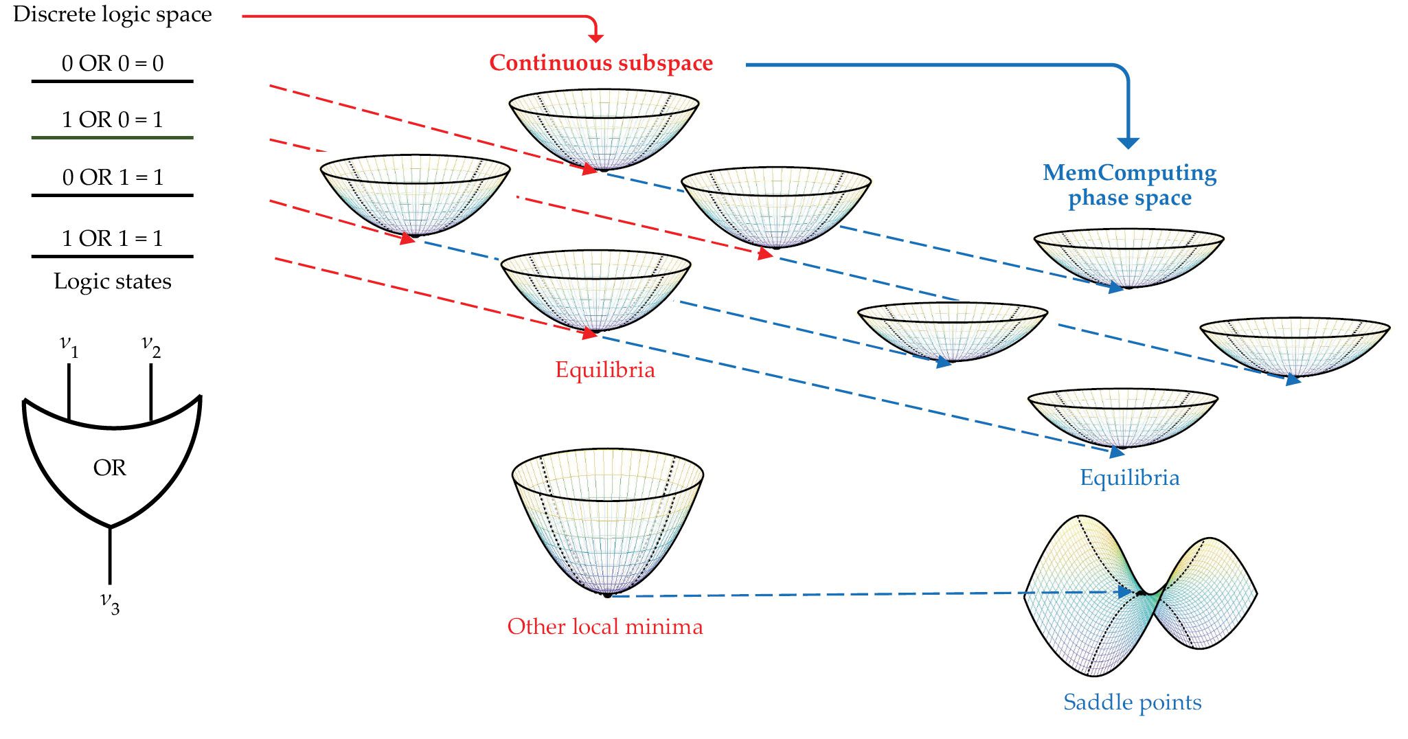
I have now transitioned from the discrete space of logic states to the continuous phase space of dynamic variables. And I can map the four logically consistent states of the OR gate into four distinct equilibrium points of the system’s dynamics. But if I stop here, the phase space may have additional local minima beside the four equilibrium points (figure 3, middle). And if the system ends up in one of those additional “wrong” local minima, it will not be able to get out and hence not solve the problem.

Here is how memory, in the form of additional dynamic variables, helps to solve that problem. If I add memory variables, which one could think of as additional degrees of freedom, I can extend the phase space of the original variables—from which I read the solution—to a larger phase space. That way, if I add the memory variables appropriately, ⁴ I can transform the local minima I don’t want into saddle points, thus opening up directions in phase space from which the system can move toward the solution (figure 3, right). It is in that enlarged phase space, containing only saddle points and equilibria representing the solutions of the problem, that the machine performs its computation.

Topological nonquantum computing

How does that computation occur? Unlike the Hilbert space of quantum computers, ³ the dimension of the phase space in a digital MemComputing machine grows linearly with the number of degrees of freedom of the system—the number of original variables v_i plus the additional memory variables. Suppose that the location of those variables is indicated with the state vector x. That dimension, in turn, grows polynomially (linearly, typically) with the size of the problem being solved. ⁷ The dynamics are then dictated by some equation of motion of the type dx/dt = F(x), with F being some appropriate function. ⁴

If that were the whole story and the dynamics were simply a random walk in phase space, the computation would not be efficient. Instead, the system can only go from one saddle point with a certain number of unstable directions—along which the machine can move toward the solution—to another saddle point with fewer unstable directions until its dynamics end in equilibria. The equilibria, which are the solutions to the problem, don’t have any unstable directions, as shown in figure 4. (Notice the lack of any downward-pointing parabolas there.)

Figure 4.

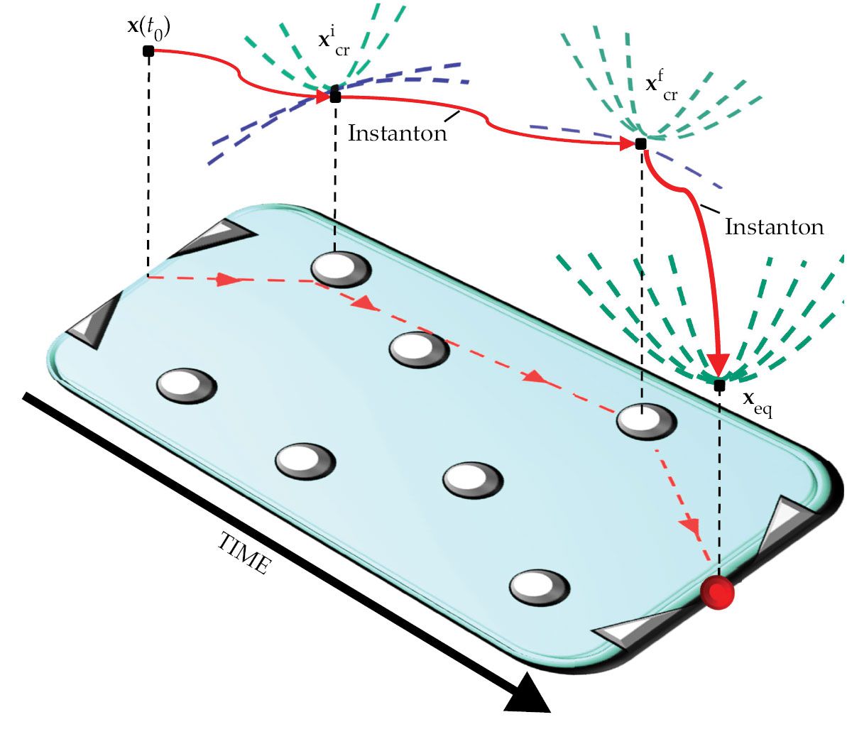
The phase-space trajectories between the saddle points—and from the last saddle point to the equilibria—have the fancy name instantons. ⁹ That’s because they connect two distinct critical points in the phase space (those where F(x) = 0), and they occur in a very short, but finite time—an instant. Instantons are the classical equivalent of tunneling between two states. And because they connect two inequivalent critical points, they are topological objects: They cannot be destroyed without changing the phase-space topology. ¹⁰ The dynamics of the MemComputing machines are thus quite robust against noise and perturbations. ⁴

In fact, the dynamics are quite similar to those of the ball in a pinball machine, in which the bumpers are saddle points and the trajectories between them are the instantons, as shown in figure 4. If one were to shake the machine, the ball might take a different path and hence follow different instantons, but it will always exit at the bottom as driven by gravity. What’s more, instantons are the type of nonperturbative phenomena that are key to compute hard problems efficiently. In fact, a single instanton can involve a large number of variables simultaneously—that is, collectively. ¹⁰

A physical system (a digital MemComputing machine) computes even difficult combinatorial-optimization problems efficiently. Every time the machine tunnels from one saddle point to another, more stable one—that is, one having a smaller number of unstable directions—via an instanton, it sheds unstable directions. The instanton brings the machine to a more stable saddle point, a process that repeats until the machine reaches the most stable point, which is the solution of the problem.

Because the number of unstable directions is at most equal to the dimension of the phase space, and the latter grows linearly with the number of degrees of freedom, the number of instantons the machine needs to reach the solution can grow at most only polynomially with the size of the problem. That statement is true even in the presence of moderate noise and perturbations. ¹⁰

Hardware and software

The physical hardware that makes up the machines can include electrical, optical, spintronic, and superconducting circuits. ⁴ Some realizations may be more advantageous than others in terms of their spatial footprint, energy consumption, and ease of integration. But in many cases, the machines’ equations of motion are ordinary differential equations. As such, they can be efficiently programmed in software so that one can test the machines’ performance by simply simulating them on a traditional computer.

Testability is a major advantage of MemComputers over quantum computers. A wide variety of combinatorial-optimization problems have already been tackled by simulating the equations of motion of the machines. ⁴ The simulations have shown considerable advantages over traditional algorithms and strongly suggest that building the machines’ hardware is achievable. In fact, for some applications of interest to industry, a software solution is sufficient. ¹¹

Epilogue

MemComputing is a physics-based approach to computation radically different from both the traditional Turing paradigm and even quantum computing. It uses time nonlocality (memory) as a tool to navigate a complex phase space efficiently. And because it relies on nonquantum dynamic systems, not only can a digital MemComputing machine be built using solid-state hardware, but it can also be efficiently simulated in software, which makes it easier to deploy in industry. The machines were originally designed to tackle combinatorial-optimization problems, but their application range also covers machine learning and quantum mechanics, which open new and interesting research directions. ⁴

The physics of the machines shares several remarkable features with nonabelian gauge theories, such as quantum chromodynamics, ¹² and the calculation of how many instantons are required to reach the solution of a given problem is an exercise in algebraic topology. ¹³ Those ideas suggest an intriguing duality between that field of mathematics and computational-complexity theory—which focuses on how one can solve combinatorial-optimization problems more efficiently—and that is worth exploring further.

References

1. D. Deutsch, The Fabric of Reality: The Science of Parallel Universes—and Its Implications, Allen Lane (1997).
2. A. M. Turing, Proc. London Math. Soc. s2-42, 230 (1937). https://doi.org/10.1112/plms/s2-42.1.230
3. M. A. Nielsen, I. L. Chuang, Quantum Computation and Quantum Information: 10th Anniversary Edition, Cambridge U. Press (2010).
4. M. Di Ventra, MemComputing: Fundamentals and Applications, Oxford U. Press (2022).
5. C. G. Langton, Physica D 42, 12 (1990). https://doi.org/10.1016/0167-2789(90)90064-V
6. M. Di Ventra, Y. V. Pershin, Nat. Phys. 9, 200 (2013). https://doi.org/10.1038/nphys2566
7. F. L. Traversa, M. Di Ventra, Chaos 27, 023107 (2017). https://doi.org/10.1063/1.4975761
8. F. L. Traversa, M. Di Ventra, IEEE Trans. Neural Netw. Learn. Syst. 26, 2702 (2015). https://doi.org/10.1109/TNNLS.2015.2391182
9. R. Rajaraman, Solitons and Instantons: An Introduction to Solitons and Instantons in Quantum Field Theory, North Holland (1987).
10. M. Di Ventra, I. V. Ovchinnikov, Ann. Phys. 409, 167935 (2019). https://doi.org/10.1016/j.aop.2019.167935
11. For more on MemComputing as a computing architecture, visit www.memcpu.com .
12. A. S. Schwarz, Quantum Field Theory and Topology, Springer (1993).
13. A. Hatcher, Algebraic Topology, Cambridge U. Press (2002).
More about the authors
Max Di Ventra is a professor of physics at the University of California, San Diego. This article is an adaptation of his book, MemComputing: Fundamentals and Applications, published by Oxford University Press.