Medical diagnostic ultrasound

As early as 250 BCE, captains of ancient Greek ships would drop lead weights overboard to provide an estimate of water depth. They would count until those “sounders” produced an audible thud and in that way measure the propagation time of the falling weight. Even though the practice has given way to other technologies for sounding, one still hears the phrase “to sound something out.” In the 17th century, Isaac Newton became fascinated with sound propagation and was one of the first to describe relationships between the speed of sound and measurable properties of the propagation medium, such as density and pressure. Section 8 of Book 2 of the Principia, for example, is devoted to “the motion propagated through fluids” and includes the proposition that the sound speed is given by the square root of the ratio of the “elastic force” to the density of the medium.

Newton’s calculations, however, contained a systematic error for which he could not account, so his estimates of sound speed were always lower than measured values. It took until the advent of thermodynamics in the 19th century for Pierre Simon Laplace and other scientists to discover that acoustic propagation is usually adiabatic rather than isothermal. That is because free propagation does not allow sufficient time for heat exchange between compressive and rarefactive portions of the sound wave. Only in the boundary layer adjacent to a solid surface is the process approximately isothermal, a fact exploited in creating refrigerators whose only moving part is a loudspeaker (see Physics Today, June 1999, page 18 ).

The dawn of ultrasound

Soon after the sinking of the Titanic, piezoelectric materials such as quartz or Rochelle salt were fashioned into acoustic sources whose thickness could be altered slightly by an imposed voltage. Thus underwater “sound navigation and ranging,” or sonar, became possible. During World War II, both sonar and its cousin radar (radio detecting and ranging) grew in military importance; after the war they became important to civilian commerce. Sonar’s familiar ping enabled vessels to use time-of-flight measurements of echoes to estimate target range and size. Modern biomedical ultrasound began during and immediately after World War II as an extension of sonar to higher frequencies and to the human body.

In the 1950s a single piezoelectric crystal was first employed in contact with skin to launch an acoustic wave into human tissue. The wave consisted of several cycles at a frequency of 20 kHz, beyond the capacity of human hearing. A series of reflections returned to the crystal at different times because of mismatches of acoustic impedance (density × sound speed) between organs or between organs and bone. The echoes were first represented in so-called A-mode (amplitude) displays as vertical deflections on the screen of an oscilloscope whose beam scanned horizontally at a constant speed; the result was a series of blips.

Because tissue absorbs acoustic energy as heat, the later the blips occur, the smaller their amplitude. Assuming the speed of sound in human soft tissue has the constant value of 1540 m/s, one can interpret the time between reflections as the distance between tissue layers, and the relative amplitude changes can convey information about the impedance mismatch between one layer and the next. Some pathologies previously diagnosable only with surgery were identified using that early, noninvasive ultrasound technology.

The 1960s saw the development of commercial ultrasound systems that exploited the mass production of cathode-ray tubes. If A-mode amplitudes are represented by the brightness of dots on a phosphor screen and the transducer that generates the ultrasound pulses scans across the tissue, a B-mode (brightness) image results. Assuming, among other things, that the speed of sound is constant allows quantitative imaging of deep tissues, as seen in figure 1. The Quick Study on page 84 of this issue discusses the various assumptions that go into ultrasound imaging and the artifacts that arise if those assumptions are violated.

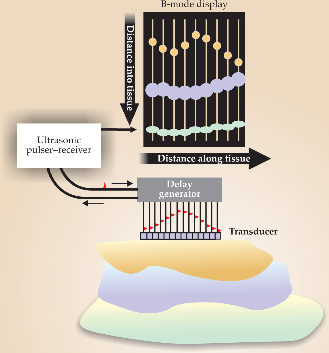
Modern ultrasound scanners use the linear superposition of spherical or cylindrical wavefronts of tiny piezoelectric crystals, usually lead zirconate titanate. Those crystals are arrayed to produce waveforms that can be steered or focused based upon the timing of the crystals’ excitations. Both the emitted and received waves may be formed by suitably manipulating timing delays and adjustable gains in the individual elements’ amplifiers. Thus a great deal of engineering goes into obtaining the image of a beating heart in an echocardiogram or of a fetus in a sonogram that may be parents’ first glimpse of their new child.

Doppler ultrasound

The Doppler effect is familiar to all who have heard the horn of an approaching train or considered the redshift of the expanding universe. In 1957 Shigeo Satomura demonstrated that the idea could be applied to ultrasound. If a sinusoidal acoustic signal of frequency f is emitted by a fixed transducer located at an angle θ with respect to a blood vessel inside of which blood cells move with average velocity V, the signals reflected to the transducer will be shifted in frequency by Δf = (2Vf/c)cosθ, where c is the speed of sound in tissue. Thus for blood cells, the Doppler shift, measured by a continuous-wave ultrasound probe transducer, can provide clinical information about blood flow.

One complication, however, is that blood is effectively a non-Newtonian fluid whose viscosity is a strong function of shear flow rate. Its sound speed varies with red blood cell concentration, which differs between capillaries and larger vessels. Because red blood cells have a diameter of only about 7 microns—much smaller than the typical acoustic wavelengths of 750 to 150 µm for 2- to 10-MHz ultrasound—they cannot be resolved individually. Instead, the 250 000 to 450 000 red blood cells in each microliter act as an ensemble and scatter back to the transducer a fluctuating pattern of constructive and destructive interference called ultrasonic speckle. Nevertheless, for a continuous-wave Doppler system, the bulk motion of the flowing red blood cells typically provides a frequency shift that falls conveniently in the audio range. The characteristic squee-choo-squee-choo sound of the Doppler audio signal from the pulsatile flow of heartbeats is common in many hospitals and obstetricians’ offices.

The biggest limitation of continuous-wave Doppler, however, is its spatial ambiguity. The difficulty arises because the Doppler signal is sensitive to all the vessels that intersect the beam. Pulsed-wave Doppler was developed in the 1970s to provide high spatial resolution; dolphins, bats, and other animals use an analogous technique to locate and identify prey. Finite-length tone bursts are emitted whose durations correspond to the size of the volume to be interrogated. Unlike the continuous-wave case, for which the Doppler-shifted received frequency is compared with the transmitted one, in pulsed-wave Doppler each received echo is compared with a similar echo from the previous transmission. Because the pulse-repetition frequency is high, only small changes in tissue geometry and absorption occur from pulse to pulse. The result is relatively high sensitivity to blood motion and relatively low sensitivity to the overall arrangement of overlaying tissues.

In the 1980s a signal-processing breakthrough allowed for the development of color flow Doppler, also called color flow imaging (CFI). At the time, clinicians knew that variations in blood-flow velocities in an interrogated volume give rise not to a single Doppler shift, but rather to a whole spectrum of shifted frequencies. Fast-Fourier-transform methods for examining the spectra were too slow and the results too variable to be clinically useful. The new CFI technique estimated the average Doppler-shifted frequency by means of the small relative phase shifts from one reflected pulse to the next.

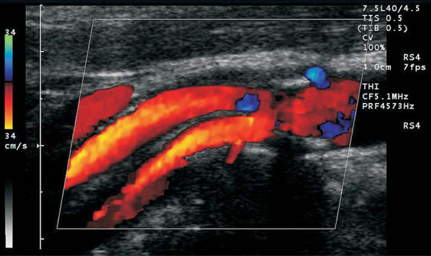
Admittedly, those phase shifts result from slightly different sets of blood cells being present in the interrogated volume from one pulse to the next and so are not, strictly speaking, Doppler shifts of individual scatterers. Nevertheless, as long as the change in scatterer distribution varies only slightly from pulse to pulse, CFI determines not only the average blood velocity but also a spectrum of velocities that can be color coded to represent forward and reverse blood flow. Such flow data are typically overlaid on the B-mode image in modern ultrasound scanners, as shown in figure 2.

One CFI variation that has found significant use in the past 10 years is so-called power Doppler, in which the integral over all frequencies of the square of the flow speed is shown as a color overlay on the B-mode image. Although information about the direction of flow is lost, the signal-to-noise ratio is increased so that power Doppler can detect tiny speeds, or speeds of tiny amounts of fluid. It can even image flow in capillaries.

Color flow imaging methods have contributed greatly to the success of ultrasound as a medically important modality. By providing a dynamic picture of blood flow, CFI Doppler has allowed physicians to diagnose leaking heart valves, vessel-blocking plaques and clots, and other abnormalities that would otherwise be difficult to detect.

Nonlinear acoustics

The stiffness of biological tissue does not obey Hooke’s law. As a consequence, the speed of sound varies locally with pressure and temperature and produces waveform distortion that compounds with propagation distance. If two waveforms with different frequencies overlap in space and time, the tissue’s essential nonlinearity produces sum and difference frequencies in the overlap region.

The acoustic nonlinearity parameter, defined as the ratio of the quadratic to the linear term in a Taylor-series expansion of pressure as a function of density, measures the deviation of the stiffness from Hooke’s law. Because the ratio is sensitive to subtle changes in material composition not reflected in acoustic impedance mismatches, a method of imaging the nonlinearity parameter could add complementary clinical information. To accomplish so-called nonlinear imaging of tissue, one can measure the strength of the sum or difference frequency by scanning a point where two ultrasound pulses intersect. For example, the sum or difference signal can be filtered and detected by a hydrophone or skin-mounted sensor. Then the location of the coincident spot can be moved. The amplitude of the signal is proportional to the tissue nonlinearity at each point.

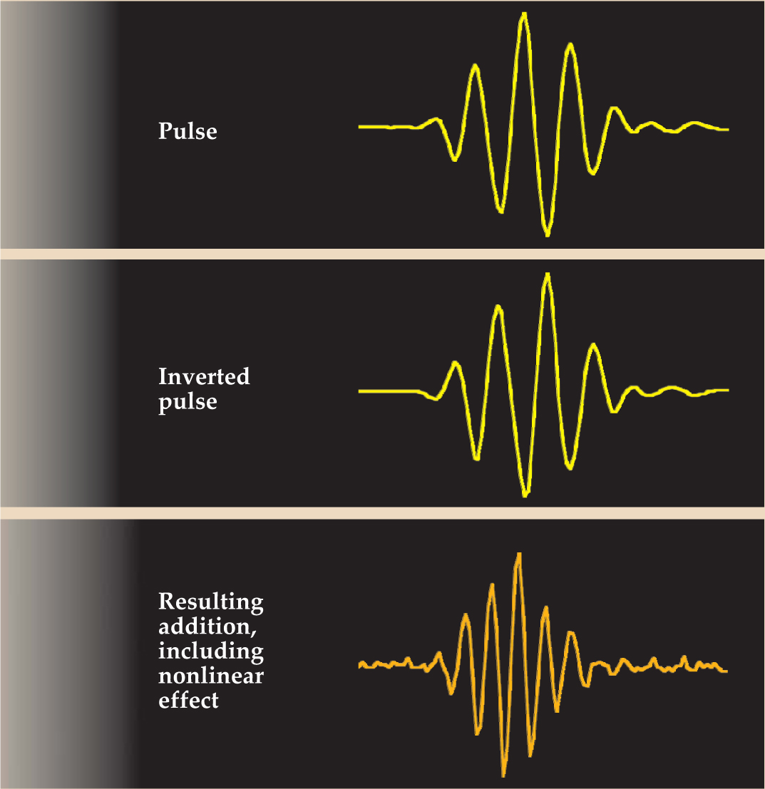
One relatively simple application of nonlinearity is tissue harmonic imaging. Developed in the late 1990s, the technique involves the combination of waveforms with the same frequency but opposite phase. Figure 3 shows a typical imaging pulse emitted from one piezoelectric element of an ultrasound transducer, with time on the horizontal axis and voltage, or pressure, on the vertical. If another array element is excited simultaneously with the inverse signal, the two pulses will mostly cancel each other’s fundamental frequency where they overlap. Tissue nonlinearities, however, tend to move energy from the fundamental up to the second harmonic, which has twice the fundamental frequency. The effect of such distortion is slightly different for the pulse and its inverse, and the result is a reinforcement of the second harmonic. The focal area of the transducer, in sum, sees a pulse with a frequency and hence spatial resolution twice that of its B-mode equivalent and reflects that pulse back to the receiving elements of the transducer. Indeed, most ultrasound scanners in use today transmit signals at one frequency and listen to the returning echoes at twice that frequency, thus achieving better spatial resolution and improved signal-to-noise ratio.

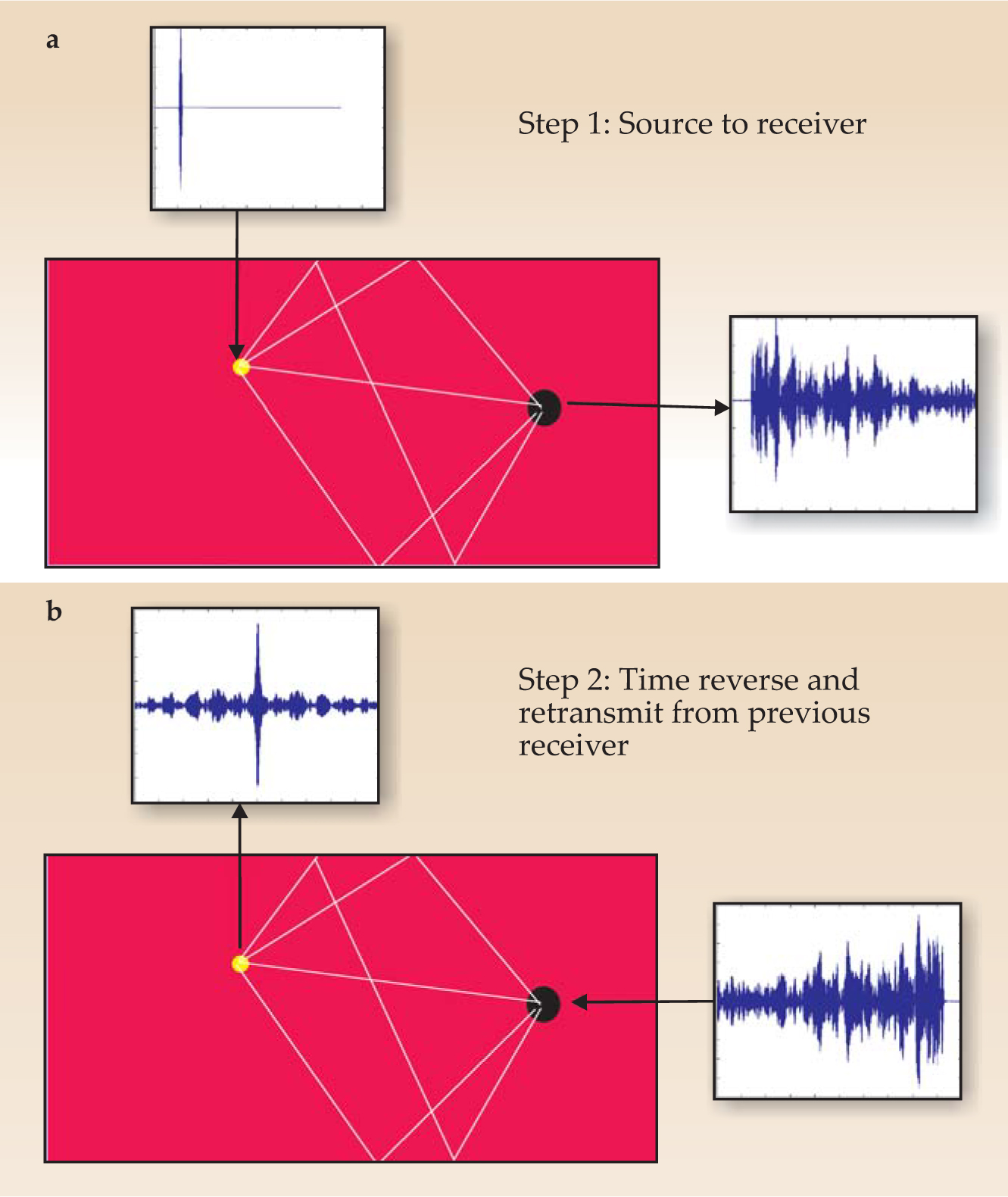
To use nonlinear superposition, large-amplitude, highly localized pulses must be made to intersect within the tissue volume. Since the late 1990s, a technique known as time-reversal acoustics (TRA) has provided a new tool to help accomplish that task. The basic idea is shown schematically in figure 4. In the first step, an acoustic source produces a pulse that propagates along many different rays to a receiver; the result is a complicated impulse response. In the second step, the pattern of pulse arrivals at the receiver is reversed, and the receiver now acts as a transmitter. Because the wave equation is time-reversal invariant, the pulses follow the step-1 rays in reverse and end up coinciding at the original source as a highly spatially and temporally focused pulse. In effect, the time-reversed signal at the receiver acts as an optimum filter to deliver subwavelength focusing at the original source location.

In practice, TRA requires that a source be placed in the body, although that source could be the tip of a biopsy needle used to reflect incident ultrasound. If the receiver is not a single transducer but many transducers mounted on a surface, a highly focused spot can be generated at the site of the original source. TRA may be combined with other modalities to further improve focusing. One therapeutic application is to brain tumors at which ultrasound is applied. In that case, computed tomography (CT) x-ray data can be used to compensate for the attenuation of the skull and the aberrations it causes to the acoustic field. Such dual-modality techniques are becoming more popular because techniques such as CT or magnetic resonance imaging provide information complementary to the mechanical parameters determined by ultrasound and thereby aid detection of pathology.

Tiny bubbles

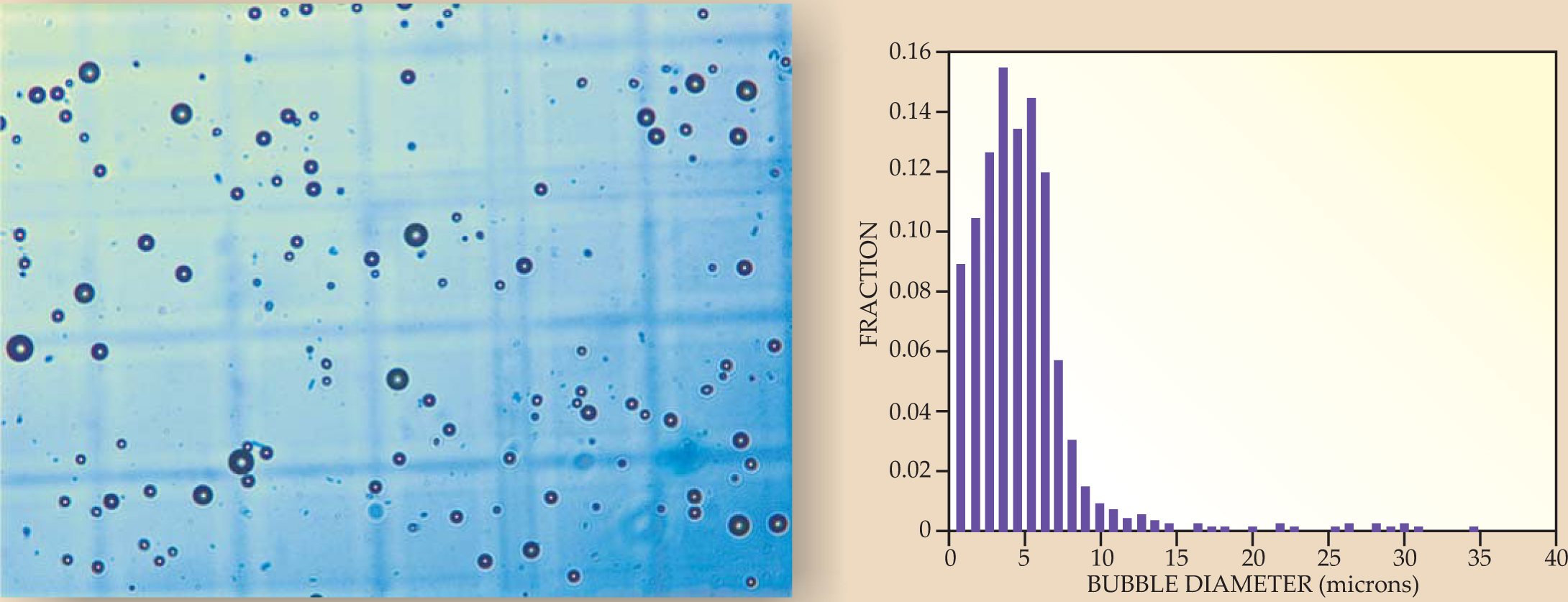
An increasingly important technique in diagnostic ultrasound involves blood-cell-sized microbubbles of perfluorocarbon gas, coated with proteins, lipids, or polymers (see figure 5). Such echo-contrast agents act as reflectors of ultrasound and are especially useful for quantifying blood flow in capillary beds or, when the bubbles’ coatings contain biochemical markers called ligands, for helping doctors identify pathologies. Indeed, clot-sticking coatings may help not only to identify stroke-causing blood clots but also to treat them, since high-amplitude ultrasound pulses may destroy bubbles and release clot-dissolving drugs.

Due to the acoustic impedance mismatch between bubbles and blood, bubbles reflect ultrasound strongly. The resulting reaction force, called the acoustic radiation force, pushes bubbles away from a transducer producing an ultrasound beam, or toward the pressure antinodes in an acoustic standing wave.

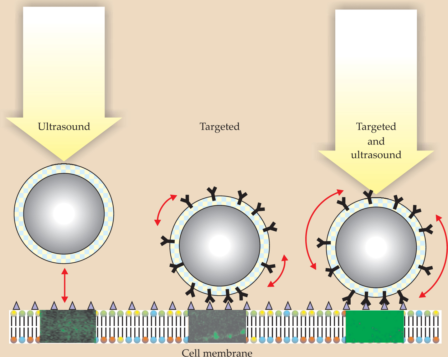
Each bubble has an acoustic resonance frequency related to the mass of the liquid around the bubble and the stiffness of the gas inside it. For an ultrasonic beam with a dominant frequency component near a bubble’s resonance frequency, the acoustic radiation force can be strong enough to push the bubble to a vessel wall where drugs in the bubble coating can be released. As shown in figure 6, the combination of ligands to help the bubbles stick to the surface with an acoustic radiation force to press and wiggle the bubbles on the vessel wall enables a dramatic improvement in drug delivery compared with the cases in which either the ultrasound or ligands are absent. A specific example of targeted drug delivery using ultrasound and bubbles is the delivery of chemotherapeutic agents to a tumor only, rather than systemically.

When a bubble is driven near resonance at a sufficiently large acoustic amplitude, its diameter can change appreciably during an acoustic cycle. If the maximum diameter is less than twice the undisturbed diameter, the bubble is said to undergo stable acoustic cavitation; its motion is mainly governed by the stiffness of the gas inside it. If the diameter more than doubles, the motion is controlled by the mass of the liquid surrounding the bubble; it undergoes inertial cavitation. Inertial-cavitation bubbles commonly implode with such force that pressures of thousands of atmospheres and temperatures of tens of thousands of kelvin occur at their centers (see the article by Detlef Lohse in Physics Today, February 2003, page 36 ). Nearby tissues can be destroyed—a result to be avoided in diagnostic applications but one that can be useful for therapy. Nowadays, microbubble–ultrasound interactions also see applications that range from breaking kidney stones with acoustic shock waves (lithotripsy) to noninvasive removal of cholesterol plaque from arteries.

If the echo-contrast bubbles span an appropriate size range, both kinds of cavitation may be present simultaneously. Because stable cavitation generates acoustic emissions below the beam frequency and inertial cavitation produces broad-bandwidth acoustic noise at the moment of implosion, bubble activity can be detected and quantified. Such monitoring may make it possible to harness the potentially destructive effects of ultrasound for new therapies while avoiding adverse bioeffects in diagnostic applications. For both therapeutic and diagnostic applications, a greater understanding of the nonlinear mechanical properties of tissues, of bubbles, and of their interactions holds the promise of more advances in the medical use of ultrasound.

References

1. F. V. Hunt, Origins in Acoustics: The Science of Sound from Antiquity to the Age of Newton, Yale U. Press, New Haven, CT (1978).
2. R. T. Beyer, Sounds of Our Times: Two Hundred Years of Acoustics, AIP Press/Springer, New York (1999).
3. T. L. Szabo, Diagnostic Ultrasound Imaging: Inside Out, Elsevier Academic Press, Burlington, MA (2004).
More about the authors
Carr Everbach is a professor of engineering at Swarthmore College in Swarthmore, Pennsylvania.
E. Carr Everbach, 1 Swarthmore College, Swarthmore, Pennsylvania, US .