Manipulating the color and shape of single photons

What does it mean to refer to a single photon? In the original conception put forth by Max Planck and Albert Einstein between 1900 and 1905, the light quantum was a carrier of a precise amount of energy. They postulated that for a given mode of the electromagnetic field with frequency ω, the energy content is an integer multiple of ℏω, with ℏ being Planck’s constant. The multiplying integer is the number of “photons,” a term coined by chemist Gilbert Lewis in 1926. Paul Dirac’s formal quantization of the electromagnetic field offered a more sophisticated view of photons. In his theory, a convenient set of eigenstates for describing photon states is defined by four quantum numbers, one for the helicity, or projection of spin along the propagation axis, and one each for the three components of momentum. Alternatively, one can specify an eigenstate by giving its polarization, its energy, and two momentum components.

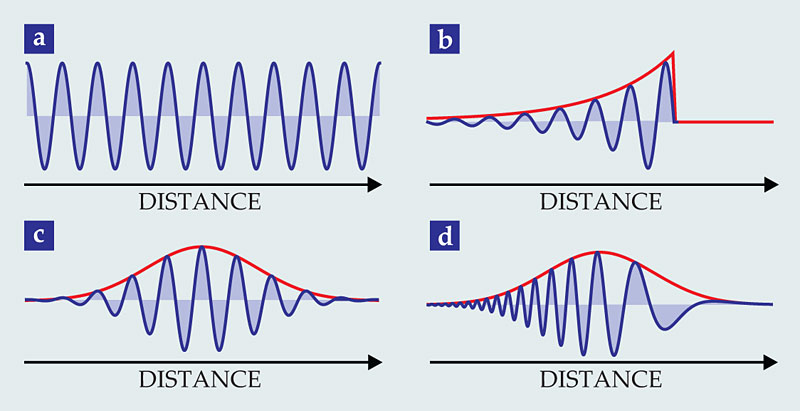
The simple eigenstates of the Dirac theory, however, are not what is created when a single excited atom decays. What is created is a superposition involving ranges of the eigenvalues described above. For example, the emitted photon will have a spread of energies given by the inverse of the atomic lifetime, in accordance with the uncertainty principle. In other words, its quantum state is a linear superposition of single-photon energy eigenstates—a coherent wavepacket with a particular temporal and spatial shape. Figure 1 illustrates several examples.

Physicists are currently working to manipulate coherent wavepacket states of single photons, which may be crucial players in a futuristic information processing and communications network—the quantum internet. ¹ Because photons interact only weakly with their environment, they are good carriers of information. Controlled manipulation of photons̵—in particular of their central frequency and their shape—will enable them to communicate between the computational nodes of the quantum internet, as described in greater detail in box 1. The endeavor is bringing together such diverse research fields as atomic physics, nonlinear optics, semiconductor physics, superconducting-circuit physics, and optomechanics.

Theory of frequency conversion

Most phenomena in nonlinear optics are based on parametric oscillations, which occur in any oscillatory system whose parameters vary periodically in time. ² In a mechanical system, for example, varying the length of a pendulum at twice the pendulum’s resonant frequency can pump energy into the resonant oscillation. In optics, the parameter to be varied is typically a medium’s electronic susceptibility, the proportionality factor relating a driving field at a specific frequency to the induced electric dipole. If strong light fields cause the susceptibility to oscillate, then energy can be redistributed between optical modes of various frequencies.

To fully describe the phenomenon, one could use a perturbation expansion that includes all powers of the strong electric field and appropriate higher-order susceptibilities as prefactors. The dominant effect is usually governed by the second-order susceptibility χ⁽²⁾ in noncentrosymmetric (lacking a center of symmetry) media such as lithium niobate or gallium arsenide crystals. In centrosymmetric media such as glass or silicon, χ⁽²⁾ vanishes and the third-order susceptibility χ⁽³⁾ typically governs.

Weak light of a given frequency ω₁ can be converted to ω₂ using either the second-order or third-order nonlinear optical response. In the second-order case, a strong laser field—the pump—modulates the medium’s susceptibility at frequency ω_p, which leads to light generation at the sum and difference frequencies ω₂ = ω₁ ± ω_p. A frequency increase is called up-conversion; a decrease, down-conversion.

To obtain a third-order nonlinear optical response, one can use two strong pump fields with frequencies ω_p and ω_q; together they modulate the medium’s susceptibility at the difference frequency δω = ω_p − ω_q. Light initially at frequency ω₁ will be up- or down-converted to the frequency ω₂ = ω₁ ± δω. That conversion process, called four-wave-mixing Bragg scattering, allows for smaller frequency shifts than can be realized in the second-order case and thereby offers distinct capabilities for designing optical interconnections between nodes in a quantum network.

In box 2, we discuss physical devices that implement quantum frequency conversion (QFC), the process of changing the frequency of a quantum state of light—for example, a single-photon state—without changing its other state properties in an uncontrolled way. Of particular importance is that photon momentum must be conserved in the course of QFC, or, in the jargon of the field, phase matching must be ensured.

Theory into practice

The quantum description of parametric nonlinear processes was developed in the 1960s by William Louisell, Amnon Yariv, and Anthony Siegman; by John Armstrong, Nicolaas Bloembergen, and colleagues; and by Yuen-Ron Shen. ³ But well more than 20 years passed before Prem Kumar pointed out that frequency conversion of quantum states of light could actually be exploited as a useful tool. ⁴ In those days Kumar was not talking specifically about single-photon QFC; rather, QFC was a process by which it was “possible to change the frequency of an input light beam while maintaining its quantum state.” By a quantum state of a light beam, Kumar was referring to a particular superposition of occupation numbers for each electromagnetic mode within some narrow range of frequencies and propagation directions.

Kumar’s work focused on second-order nonlinear processes for achieving QFC, and for many years afterwards QFC was almost exclusively discussed in that context. However, in 2005 Colin McKinstrie and colleagues showed theoretically that QFC could be achieved via four-wave-mixing Bragg scattering; ⁵ that demonstration opened up the application to whole new classes of materials, notably glass optical fibers and silicon photonic devices.

One application of QFC, envisioned relatively early, was in developing a tunable source of squeezed light. In quantum optics, squeezing is a process by which the fluctuations in some observable quantity such as the electric field amplitude are reduced to a level below that allowed in a classical theory of optical fields, albeit at the expense of increased fluctuations in the complementary observable. Squeezed states of light have found applications in interferometry, in which the noise reduction in one observable can lead to improvements in precision measurements such as those needed in the Laser Interferometer Gravitational-Wave Observatory (see Physics Today, November 2011, page 11 ). With the help of QFC, a physicist could, in principle, generate squeezed light in a system optimized for squeezing, then convert the light’s wavelength to the one most suitable for the interferometer. Indeed, in 1992 Kumar and Jianming Huang took a squeezed state of light that exhibits highly correlated, classically forbidden intensity fluctuations between two optical beams; applied QFC techniques to up-convert one beam to a new frequency; and showed that they could preserve the nonclassical correlations. ⁶

Another reason one might want to change the wavelength of a quantum state of light is to improve the ability to detect it; with QFC it is possible to shift the wavelength from a regime for which existing detectors have low performance—in terms of detection efficiency, speed, or noise—to a range for which better options exist. The idea is not new: In the 1960s several groups used frequency up-conversion to enable conventional photomultipliers to detect IR light from, for example, carbon dioxide lasers and astronomical objects. More recently, groups such as those of Martin Fejer and Paul Kwiat have considered QFC as a means by which visible-wavelength detectors could see photons created in the telecommunications wavelength windows around 1.55 µm and 1.3 µm, where loss and dispersion are minimized in optical fibers. ⁷

Frequency conversion of single photons

Driven in part by potential applications in quantum information technology, researchers have developed an ever-increasing set of approaches for generating various quantum states of light. Some of those states have been used in experimental demonstrations of QFC. For example, in many quantum information protocols, entanglement is a central resource. An entangled state of two spatially separated systems is nonseparable—that is, not expressible as a product. In 2005 Sébastien Tanzilli and coworkers performed QFC on one member of a pair of entangled photons and showed that a form of entanglement, called time-bin entanglement, is preserved even after one photon of the pair is up-converted from the telecommunications band to the visible. ⁸ Last year a similar experiment by Nobuyuki Imoto and colleagues demonstrated the opposite process in which entanglement is preserved when one photon of the pair is down-converted from the visible to the telecommunications band. ⁹

Recent efforts have focused on the preservation of the number statistics of single-photon states. In 2010 Hayden McGuinness and coworkers demonstrated single-photon QFC via four-wave-mixing Bragg scattering in optical fibers; in their experiment, they shifted the wavelength of single photons by 24 nm. ¹⁰ At the same time, Matthew Rakher and colleagues used the second-order nonlinearity in a crystal to up-convert single-photon states by nearly 600 nm, from the telecommunications band to the visible. ¹¹ Subsequent work by the Imoto collaboration showed the reverse process of single-photon down-conversion. ⁹

Before performing QFC, one needs to generate single-photon states in a controlled manner. As discussed in box 3, that has been done by a variety of mechanisms in different physical systems. (Physicists, though, continue to explore novel mechanisms for enabling single-photon generation; see, for example, Physics Today, July 2012, page 14 .) After performing QFC, one needs to establish that the result is a single-photon state. The key effect used to do so—called photon antibunching and first demonstrated by H. Jeff Kimble, Mario Dagenais, and Leonard Mandel ¹² in 1977—is also described in the box.

In the recent QFC experiments described above, photon antibunching measurements confirmed that the single-photon character of the quantum states was preserved after frequency conversion. ^9–11 Theoretical expectations notwithstanding, practical, high-fidelity single-photon QFC is remarkable, given that the average power in the pump fields can be 15 orders of magnitude greater than that of the single-photon states: One might well worry that some experimental nonideality would ruin the single-photon character of the frequency-converted light. Indeed, the devices used for QFC suffer from a variety of unwanted background processes, typically associated with the strong pump fields, and those processes generate photons that get frequency converted along with the desired quantum state. Rejecting such noise while maintaining high overall efficiency in the QFC setup is an important goal; at present, researchers have achieved efficiencies of about 50%.

In a noteworthy experiment conducted a couple of years ago, Alexander Radnaev and colleagues showed that quantum memory elements could be interfaced with telecommunications light. ¹³ In that work, an atomic system that supports both near-IR and telecommunications-band optical transitions enabled frequency up- and down-conversion. An excitation written into an atom-based memory was mapped, via coherent laser control, to a 780-nm wavelength photon, which was then down-converted to the 1300-nm telecommunications band in the atomic QFC medium. The photon then traveled along more than 100 m of optical fiber before being up-converted back to 780 nm in the same atomic QFC medium and mapped back into the quantum memory.

Many groups are working to go beyond performing QFC between the visible and telecommunications bands and to interconvert microwave and visible light. Part of their motivation is the many impressive quantum information processing elements designed to operate in the microwave region and the demonstrations of their success—with, for example, superconducting qubits coupled to coplanar waveguide resonators or to nanomechanical oscillators. ¹⁴ Microwaves are suitable for quantum information transfer on a single computer chip, but transfer over larger distances will likely require that they be converted to optical wavelengths, for which optical fibers offer low-loss transmission. Among the approaches being considered for microwave-to-optical conversion are the use of conventional nonlinear materials and of atomic and molecular systems that support both microwave and optical transitions. One novel strategy is to employ optomechanical systems in which microwave and optical cavities are coupled to a common mechanical oscillator that acts as an intermediary (see the article by Markus Aspelmeyer, Pierre Meystre, and Keith Schwab in Physics Today, July 2012, page 29 ). Such a scheme can enable conversion even though the microwave and optical fields never directly interact.

Getting photons into shape

In addition to its central frequency, a single-photon wavepacket is characterized by its shape; see figure 1 for examples. When a photon undergoes frequency conversion, its shape may be altered as a result of changes in its spectral content and phase structure. That reshaping can be controlled and put to good use. For example, a quantum-memory element such as an atom, ion, or quantum dot typically emits a photon wavepacket with an exponentially decaying tail, as shown in figure 1b. For propagation in a fiber or for writing into a different memory, one may need to convert that shape into a Gaussian packet or an exponential packet with a decay or growth constant that differs from the original one.

Various techniques that don’t involve frequency conversion can reshape photons. However, we will focus on those techniques for which the frequency does change. Suppose, for example, that a node of the quantum internet emits wavepackets with a relatively long duration, but the receiving node will efficiently absorb a photon only of much briefer duration. One way to convert a longer-duration wavepacket into a shorter one while also converting its frequency is to pump an up-conversion process with a strong laser pulse whose duration matches that of the desired photon. If the pump, initial, and final pulses all travel with the same group velocity, then the up-conversion process simply slices a short segment of the original photon wavepacket and converts it to a higher frequency. Indeed, as illustrated in figure 2a, Rakher and colleagues applied that technique to convert a 1300-nm photon with an exponentially decaying profile and time constant of 1.5 ns into a 710-nm photon with a Gaussian profile and duration of 350 ps. ¹⁵ Photons are indivisible, and so the procedure yields a quantum superposition of a photon with the original frequency and one with the up-converted one. Once the frequency of the photon is irreversibly measured, though, only one component survives.

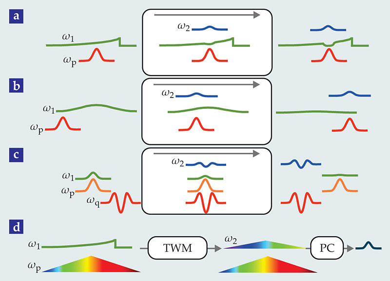
Because the process just described involves an up-converted portion being sliced from the original packet, the overall efficiency of the process can’t exceed the ratio of the durations of the final and initial packets. In some cases, though, researchers need to achieve almost perfectly efficient QFC while significantly altering the duration and shape of the photons’ wavepackets. Experimental studies toward that end are in their infancy, but several promising theoretical proposals have already been developed. A key step for achieving efficient shaping of single-photon waveforms is to tailor the dispersion of the frequency-conversion device so that the incoming photon travels through the nonlinear medium at a different speed than does the converted photon. As proposed by Christine Silberhorn and coworkers and shown in figure 2b, if a short pump pulse is initially behind a longer initial-photon wavepacket but eventually catches up to and passes through it, then the up-conversion process can sweep out all the initial-photon amplitude and efficiently compress it into a shorter, frequency-converted packet. ¹⁶ Conversely, if the initial photon packet is initially behind a longer pump pulse and then catches up to and passes through the pump pulse, the up-converted packet can be stretched.

Single-photon packet compression or stretching can also be accomplished via four-wave-mixing Bragg scattering. ¹⁷ As shown in figure 2c, the strategy is to match the initial photon wavepacket shape to that of one of the pump pulses—pulse p in the illustrated example. The dispersion properties must be tailored so that the initial photon wavepacket travels with the same group velocity as the initially matched pump pulse and the frequency-converted photon travels with the same group velocity as the other pump pulse—q in the figure. Then the frequency-converted photon takes on roughly the shape of the other pump pulse, a shape that can be quite different from that of the initially matched pulse.

A fourth type of photon-reshaping scheme, proposed by David Kielpinski and colleagues, ¹⁸ is shown in figure 2d. If the pump pulse is appropriately tailored in spectrum and temporal phase, then those characteristics will be transferred to the converted photon. In the example shown, the pump has a time-varying frequency and the original signal photon is a negative exponential with a fixed frequency. Upon up-conversion, the new signal photon has a temporally varying frequency; it can then be compressed and shaped via a dispersive delay line, typically made with diffraction gratings.

The schemes illustrated in figure 2, and others, allow for defining photonic qubits based on color or shape. A single photon could be created in a superposition of two colors—for example, red and green. Or a photon could be created in a superposition of two distinct wavepacket shapes that overlap in time and have the same central frequency.

Color, shape, and quantum information

These days many quantum-information physicists are excited about learning how to manipulate the frequencies and shapes of single-photon wavepackets, operations that can be critical to quantum information networks. The essential physical resource for enabling quantum information systems to outperform classical ones is quantum entanglement. Therefore, we need to learn how to control, across wide ranges of the spectrum, the entanglement of quantum states involving material and photonic qubits. And doing so with high efficiency, fidelity, and low background noise remains challenging.

In general, for QFC via second-order nonlinear processes, we need crystals and devices with tailorable dispersion properties so that we can efficiently convert a photon’s frequency while altering its duration and shape to the desired form. For QFC by third-order processes, we need optical fibers that are more uniform along their length. Moreover, the quantum internet of the future will likely comprise a large number of nodes and may require a large number of QFC interfaces that consume significant resources. For that reason, researchers are working to make practicable the implementation of QFC by microchip-scale devices. If physicists succeed in meeting those challenges, we can all look forward to an internet whose fundamental physical character and capabilities vastly differ from that of our current technology.

Box 1. The quantum internet

The idea behind quantum information processing is to use quantum superposition states to transmit, store, and process information. Instead of using the classical bit, which can be either 0 or 1, quantum information processing exploits the qubit, an object that can be prepared in a coherent superposition of states representing 0 and 1. The additional structure in the qubit leads to computational and communications abilities that do not exist with classical hardware.

Many physicists, including the two of us, think it unlikely that future quantum information processors and communication systems will be composed of units based on a single type of physical system such as a particular kind of atomic ensemble, trapped ion, semiconductor, or superconductor. Instead, we expect a hybrid network to emerge, in which different types of physical systems play different roles. The quantum internet we imagine will include computational nodes containing atoms or superconductors, for example, that act as quantum memories or processors. To communicate quantum information, each node will absorb and emit photons at its own natural resonance frequency and line shape. That diversity of colors and forms creates a challenge: how to convert a single photon from one frequency to another and alter its wavepacket shape to fit optimally with different material systems. It is as if two types of quantum nodes were speaking a different language and one needed a translating device to get the message across.

The figure illustrates this notion of translation. In it, a pair of quantum frequency conversion (QFC) devices connect a quantum dot operating at photon frequency ω₁ to an atomic vapor operating at frequency ω₂ through an optical fiber that optimally transmits light at frequency ω₃. The eventual goal is to spread quantum-state entanglement throughout a large network of memories or processors.

Box 2. Devices for quantum frequency conversion

Over the past five decades, physicists working in nonlinear optics have established that it is possible to change the frequency of a single photon with nearly 100% efficiency without changing the photon’s other state properties in an uncontrollable manner. That achievement represents an improvement of eight orders of magnitude over the efficiency demonstrated some 50 years ago in the first experimental work in nonlinear optics—the second-harmonic generation experiments of Peter Franken and coworkers. The vast improvement is the result of efforts to identify materials with large nonlinear optical coefficients, the use of strongly confining waveguides to increase optical intensities and enhance effective nonlinearities, and the application of new methods to achieve the requisite phase matching—in essence, momentum conservation among photons. (See the article by Martin Fejer, Physics Today, May 1994, page 25 .)

Phase matching plays a crucial role in nonlinear optics. In vacuum, it is guaranteed because the photon frequency ω and wavevector k ≡ ω/c, which plays the role of momentum, are related simply by the speed of light. In materials, however, phase matching is not guaranteed because matter exhibits dispersion—light at different wavelengths propagates at different speeds.

The figure shows examples of devices that enable up-conversion—that is, an increase in the frequency of a single photon. In the upper panel, the up-conversion is governed by the second-order susceptibility χ⁽²⁾. The second-order material, in conjunction with a strong pump laser at frequency ω_p, converts input photon pulses at ω₁ to output pulses at ω₂ = ω₁ + ω_p. A uniform material would not satisfy phase matching, because k₂ ≠ k₁ + k_p. Thus the illustrated device uses quasi-phase matching (QPM); as shown below the device in the panel, a spatially periodic change (with period Λ) in the material properties of the nonlinear medium compensates for the momentum mismatch.

The lower panel shows a highly nonlinear fiber (HNLF), in which the up-conversion is governed by the third-order susceptibility χ⁽³⁾. Input single-photon pulses at frequency ω₁ combine with strong pump lasers at ω_p and ω_q to generate up-converted single-photon pulses at ω₂ = ω₁ + ω_p − ω_q. In this case, phase matching is achieved by compensating for the material’s natural dispersion by so-called waveguide dispersion, which arises as a consequence of the detailed construction of the HNLF: The fiber consists of a central core region and a surrounding cladding region, each having different material properties. As a result, the exact distribution of the optical field within the fiber, and thereby the light’s phase velocity, depends on wavelength. Furthermore, the HNLF confines light to a very small cross-sectional area. That, in combination with new materials, increases the effective nonlinearity relative to a standard silica fiber.

Box 3. Creating and confirming single photons

A simple way to generate single-photon states is to strongly attenuate a laser pulse. That approach has a fundamental limitation, however, because the number of photons put out by the laser follows a Poisson distribution. As illustrated in panel a of the figure, for an average photon number of 1, the probability of having two or three photons is high; limiting the multiphoton probability requires a much weaker pulse, with an average photon number of 0.1 or so. In that case, however, the single-photon probability is also small, and most pulses contain no photons.

Nonlinear optics provides an improved approach to generating single photons. Certain types of materials—for example, highly nonlinear fibers (HNLFs)—allow for the process of photon pair generation, as illustrated in panel b. Here, two pump photons at frequency ω_p are converted to a pair of simultaneously emitted photons at frequencies ω_i and ω_s. Generation of photon pairs is probabilistic, however, so it is impossible to know exactly when the pairs are generated. But because the photons are produced in pairs, spectrally separating the pair and detecting one of the two—a process called heralding—provides assurance that the partner photon is present.

A third approach to single-photon generation is illustrated in panel c. It uses single-quantum emitters, materials in which a single radiative transition can be isolated. Such systems include single atoms, ions, quantum dots, and molecules. Laser pulses prepare the system in an excited state, and when the system relaxes to its ground state, it emits a photon. In principle, a single photon should be produced with each excitation pulse; the two detectors shown in the illustration, for example, should never trigger simultaneously. Sources based on the approach described in this paragraph are called on-demand or triggered single-photon sources.

To confirm the production of single-photon states, researchers perform a type of photon-number correlation measurement that was first applied to stellar interferometry by Robert Hanbury Brown and Richard Twiss in the 1950s. As schematically depicted in panel c of the figure, a beamsplitter divides incoming light equally into two paths, each directed to a single-photon detector, which records the arrival times of incident photons. Those measurements are then used to generate a histogram of the difference in arrival times between photons in the two paths. If isolated single photons impinge on the beamsplitter, at most one of the detectors will observe a photon at any given time. As a result, the histogram should show an absence of coincidences at zero time delay—an effect called photon antibunching. In the graph of the time-dependent correlation function g⁽²⁾(τ), the antibunching is manifested by the absence of a tall peak at zero time delay.

Hanbury Brown and Twiss measurements may also be used to characterize other quantum light sources. Some sources, for example, generate a pair of photons at the same instant; a Hanbury Brown and Twiss measurement will show a much greater number of coincidences at zero time delay than at other delays. Laser light, on the other hand, shows an equal number of coincidences across all time delays. Coincidence counting thus allows for discrimination among different quantum states of light that might have the same average power when measured with a standard optical detector.

References

1. H. J. Kimble, Nature 453, 1023 (2008); https://doi.org/10.1038/nature07127
S. Lloyd et al., Comput. Commun. Rev. 34 (5), 9 (2004); https://doi.org/10.1145/1039111.1039118
J. L. O’Brien, A. Furusawa, J. Vučković, Nat. Photonics 3, 687 (2009). https://doi.org/10.1038/nphoton.2009.2292. See, for example, R. W. Boyd, Nonlinear Optics, 3rd ed., Elsevier Academic Press, Burlington, MA (2008);
G. P. Agrawal, Nonlinear Fiber Optics, 4th ed., Elsevier Academic Press, Burlington, MA (2007).3. W. H. Louisell, A. Yariv, A. E. Siegman, Phys. Rev. 124, 1626 (1961);
J. A. Armstrong et al., Phys. Rev. 127, 1918 (1962); https://doi.org/10.1103/PhysRev.127.1918
Y. R. Shen, Phys. Rev. 155, 921 (1967). https://doi.org/10.1103/PhysRev.155.9214. P. Kumar, Opt. Lett. 15, 1476 (1990). https://doi.org/10.1364/OL.15.001476
5. C. McKinstrie et al., Opt. Express 13, 9131 (2005). https://doi.org/10.1364/OPEX.13.009131
6. J. Huang, P. Kumar, Phys. Rev. Lett. 68, 2153 (1992). https://doi.org/10.1103/PhysRevLett.68.2153
7. See, for example, A. P. Vandevender, P. G. Kwiat, J. Mod. Opt. 51, 1433 (2004); https://doi.org/10.1080/09500340408235283
C. Langrock et al., Opt. Lett. 30, 1725 (2005); https://doi.org/10.1364/OL.30.001725
E. Diamanti et al., Opt. Express 14, 13073 (2006). https://doi.org/10.1364/OE.14.0130738. S. Tanzilli et al., Nature 437, 116 (2005). https://doi.org/10.1038/nature04009
9. R. Ikuta et al., Nat. Comm. 2, 1544 (2011). https://doi.org/10.1038/ncomms1544
10. H. J. McGuinness et al., Phys. Rev. Lett. 105, 093604 (2010). https://doi.org/10.1103/PhysRevLett.105.093604
11. M. T. Rakher et al., Nat. Photonics 4, 786 (2010). https://doi.org/10.1038/nphoton.2010.221
12. H. J. Kimble, M. Dagenais, L. Mandel, Phys. Rev. Lett. 39, 691 (1977). https://doi.org/10.1103/PhysRevLett.39.691
13. A. G. Radnaev et al., Nat. Phys. 6, 894 (2010). https://doi.org/10.1038/nphys1773
14. R. J. Schoelkopf, S. M. Girvin, Nature 451, 664 (2008); https://doi.org/10.1038/451664a
A. D. O’Connell et al., Nature 464, 697 (2010). https://doi.org/10.1038/nature0896715. M. T. Rakher et al., Phys. Rev. Lett. 107, 083602 (2011). https://doi.org/10.1103/PhysRevLett.107.083602
16. B. Brecht et al., New J. Phys. 13, 065029 (2011). https://doi.org/10.1088/1367-2630/13/6/065029
17. C. J. McKinstrie et al., Phys. Rev. A. 85, 053829 (2012). https://doi.org/10.1103/PhysRevA.85.053829
18. D. Kielpinski, J. F. Corney, H. M. Wiseman, Phys. Rev. Lett. 106, 130501 (2011). https://doi.org/10.1103/PhysRevLett.106.130501
More about the authors
Michael Raymer is a Philip H. Knight Professor of Liberal Arts and Sciences in the physics department at the University of Oregon in Eugene. Kartik Srinivasan is a project leader in the Center for Nanoscale Science and Technology at the National Institute of Standards and Technology in Gaithersburg, Maryland.