Magnetic field reconnection: A first-principles perspective

On 28 October 2003, a large group of sunspots in the Sun’s southern hemisphere erupted, producing an intense x-ray flare and a large, fast coronal mass ejection (CME). That solar flare, like many others, released on a time scale of minutes as much as 10²⁵ joules of electromagnetic energy—roughly equivalent to all the energy stored in fossil fuels on Earth, or 10 million times as much energy as that released from a volcanic explosion. Surprisingly, up to 50% of that energy can appear as accelerated electrons. Flares also accelerate ions near the Sun to energies greater than 100 MeV.

The day after the October solar event, the CME slammed into Earth’s magnetic field and triggered a powerful geomagnetic storm during which electrons were accelerated to relativistic energies inside Earth’s radiation belts. Strong, geomagnetically induced currents over northern Europe caused the electrical grid to fail, which triggered a subsequent blackout on the ground. NASA officials issued a flight directive for space-station astronauts to take precautionary shelter. Airlines meanwhile deviated from their high-latitude routes to avoid the high radiation levels and communication-blackout areas. NASA would later report that approximately 59% of its Earth and space science missions were affected and global positioning systems disturbed.

The conversion of electromagnetic energy to accelerated particles near the Sun and in the terrestrial magnetosphere during that and many similar events occurs with efficiencies that are large and time scales that are short compared with those associated with classical collisional dissipation. Magnetic field reconnection is often invoked as the trigger that ultimately releases the energy from the magnetic field through a variety of processes. The concept of reconnection was first suggested more than a half century ago by Ronald Giovanelli as a mechanism for particle acceleration in solar flares, and the specific term “magnetic reconnection” was introduced a few years later by James Dungey in connection with particle acceleration in Earth’s magnetosphere. ^{1 , 2}

Magnetic field reconnection is thought to operate in active galactic nuclei, magnetars, pulsars, gamma-ray bursts, stellar coronae, and planetary magnetospheres. The purpose of this article is to discuss magnetic reconnection from first principles in order to explain how it works and what it is capable of doing. Of the many topics of current interest in reconnection physics, this article will focus on the mechanisms for accelerating charged particles and will discuss reconnection between solar and terrestrial magnetic field lines. (For a more complete discussion of recent research advances, see reference .)

Field-line motion

Magnetic field reconnection occurs when two magnetized plasmas, having a sheared magnetic field across their interface, flow toward each other.⁴ Its characteristic feature is a modification of the original magnetic field topology because of the presence, within some relatively small region, of dissipative processes that convert electromagnetic energy to plasma energy. One inflowing plasma and magnetic field becomes connected to the other as a result of the topological change due to reconnection.

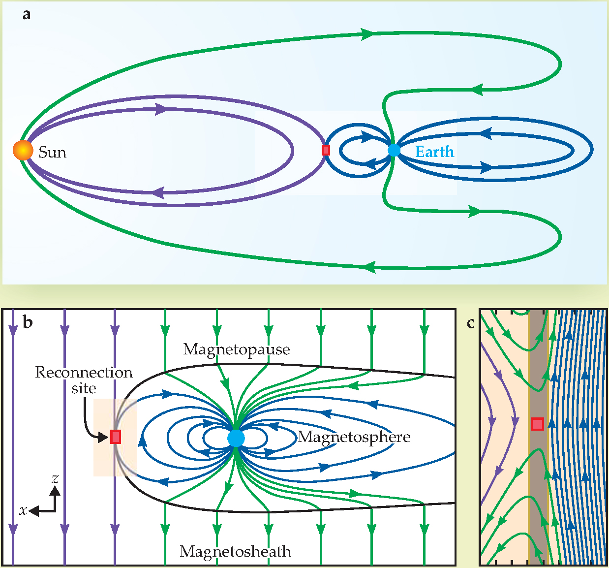
An example of the geometry of reconnection and its associated topological change is shown in figure 1. Reconnection may occur at all longitudes and latitudes, depending on the geometry, but for simplicity we show the interaction between the solar and terrestrial fields near the equator. At the reconnection site, the two fields of opposite polarities combine, a process that accelerates the plasma along the newly connected field lines.

So far, we’ve assumed that magnetic field lines flow with the plasma in which they are embedded. But do they really move? That question is as meaningless as asking whether magnetic field lines really exist, because no experiment can be devised to test either question. If the interpretation of a result is made easier by imagining that magnetic field lines exist and that they move, one may certainly use those constructs, provided that Maxwell’s equations aren’t violated. For example, one can imagine measuring the magnetic field vector everywhere in space at a given time and then tying the vectors together to make lines whose direction is the local direction of the magnetic field and whose local density is proportional to its strength.

Can one imagine those field lines moving in a way that reproduces the temporal evolution of the magnetic field geometry found by solving Maxwell’s equations? To consider the question, assume that magnetic field lines move with the velocity E × B/B ², where E and B are the electric and magnetic field vectors in the frame of interest. If that velocity causes the magnetic field geometry to evolve in the same way as do solutions to Maxwell’s equations—which will be shown to be true for a special case—then the concept of moving magnetic field lines provides a comparatively useful simplification.

Under what conditions does the construct of field-line motion produce the same solution? Assuming that two points a and b on the same field line move at the E × B/B ² velocity to points a′ and b′, the condition that the field-line direction is preserved in this motion is that (a’ − b′) is parallel to B; that is, B x(a′ − b′) = 0.

After working through the vector algebra, that condition becomes

$$B\times \left(\nabla \times E_{\text{1}}\right)=0,$$ ((1))

where ${\text{E}}_{\text{1}}\equiv \text{B}\left(\text{E}\cdot \text{B}/B^2\right)$ is the component of the electric field parallel to the local magnetic field—henceforth called the parallel electric field. ⁵ When this condition is satisfied, the movement of magnetic field lines at the E × B/B ² velocity produces the same result as do Maxwell’s equations. Interestingly, the result does not depend on the presence of plasma. However, if plasma is present, and because low-energy plasma also flows at the E × B/B ² velocity, one may visualize the plasma and magnetic field lines moving together in what is called the frozen-in condition.

An idealized case

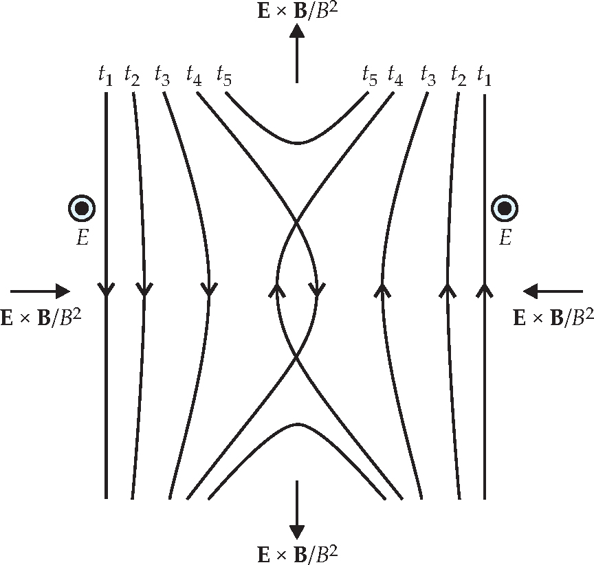
Consider the idealized case of two planar magnetic fields having a 180-degree shear between them—one field line pointed up, the other down—and an electric field pointed out of the plane, as illustrated in figure 2. Electromagnetic energy appears to be converted to plasma kinetic energy in this picture because there exist, out of the figure’s plane, an electric field and a current density j associated with $\nabla \times B,\hspace{0.17em}\text{so}\hspace{0.17em}j\cdot E>\text{0}$ . To relate the energy conversion to magnetic field reconnection, simply trace the pair of magnetic field lines in time, one moving rightward, the other leftward. But that tracing, under the assumption of zero ${\text{E}}_{\left|\right|}$ , leads to the nonphysical result in which the magnetic field points in two directions at a single point in space.

One way to avoid that result is for there to be no E component out of the plane in the central region of figure 2, so that field lines do not flow together. That scenario would produce a tangential discontinuity in which any flow in the central region is normal to the plane of the figure and reconnection does not occur. Another way to avoid a nonphysical result is for equation (1) to be unsatisfied in the central region. In that case, one can no longer assume that field lines advance at the E × B/B ² velocity. Thus, for reconnection to occur, there must be a nonzero E _|| that violates equation (1).

To understand the origin of that parallel electric field, consider the electrons and ions as fluids whose physical properties are obtained as the average of single-particle properties over small spatial volumes. Newton’s second law for such an electron fluid is $$n_e{m}_e\left[\partial U_e/\partial t+\left(U_{\text{e}}\cdot \nabla \right)U_{\text{e}}\right]=-e{n}_e\left(E+U_{\text{e}}\times B\right)-\nabla \cdot P_{\text{e}}+P_{\text{ei}},$$ ((2))

where U _e is the electron fluid velocity; n _e and m _e are the electron density and mass, respectively; e is the magnitude of the elementary charge; P _e is the electron pressure tensor; and P _ei is the momentum transferred to electrons from ions per unit volume per unit time.

A similar equation exists for ions. Subtraction of the ion equation from equation (2) yields a generalized Ohm’s law, which, after linearization and the removal of small terms, may be written as

$$E=-U_{\text{e}}\times B-\nabla \cdot P_{\text{e}}/en+\left(m_e/n{e}^2\right)\partial j/\partial t+\eta j,$$ ((3))

where η is the resistivity that arises from the exchange of momentum between electrons and ions, and n is the plasma density. ⁶ The second, third, and fourth terms on the right side of this equation are called, respectively, the pressure term, inertia term, and resistivity term. If they are all zero, E _|| is also zero because the first term on the right is perpendicular to B. In that case, the ion fluid velocity U_i = U _e = E × B/B ² and the ion fluid, the electron fluid, and the magnetic field lines move together in what is known as ideal magnetohydrodynamics (MHD) —an approximation that combines the single-fluid equations and Maxwell’s equations to describe a plasma as a conducting fluid.

Because the U _e × B term of equation (3) is not associated with a parallel electric field, the nonzero E _|| required for reconnection must come from parallel components of (in their order of importance) the divergence of the electron pressure tensor, electron inertia, or resistivity. The violation of equation (1) in the central region of figure 2 because of those terms is what allows magnetic field lines to reconnect. The energy gained from reconnection propels the inflowing plasma upward or downward out of the region.

Particle-in-cell simulations

Because it is not possible to obtain the magnetic field topology of reconnection by thinking of magnetic field lines moving at the E × B /B ² velocity through the region where they intersect, researchers must resort to simulations that produce a self-consistent solution of coupled partial differential equations—Maxwell’s equations and Newton’s second law—with given initial conditions. While different simulations have used different approximations—ideal, resistive, and two-fluid MHD and others—one particularly successful technique is that of particle-in-cell (PIC) simulations of plasmas. ^{7 , 8} In that technique, the orbits of a large number of charged particles—currently as many as 200 billion—are computed in self-consistent electric and magnetic fields.

The term “particle-in-cell” refers to the fact that the particle charges and velocities are accumulated on a spatial grid and the resulting charge and current densities are used in the solution of Maxwell’s equations. The cost of such a simulation is then proportional to the number of particles N rather than to N 2, as would be the case for a direct evaluation of the forces between pairs of particles. The PIC approach, unlike MHD, makes no approximations to the basic physics determining the behavior of collisionless plasmas. Computational limitations, though, necessitate a number of compromises in the choice of physical parameters, such as the ion-to-electron mass ratio m/m _e. For example, the computational-time cost of a simulation scales as (m/m _e)² with a two-dimensional spatial grid and as (m/m _e)^5/2 with a 3D grid. Thus a computation that requires a week of computer processing time with m/m _e = 200 would require 1.6 years in two dimensions and 4.9 years in three dimensions with the true proton-to-electron mass ratio of 1836.

Figure 3 and figure 1(c) show the results of a 2D PIC simulation ⁹ using a mass ratio of 200. At the subsolar magnetopause, where field lines from the solar wind meet Earth’s field lines, the plasma density n is about 10 cm^-3 and the proton inertial length c/ω _pi about 75 km; c refers to the speed of light and ω _pi to the ion plasma frequency (ne ²/ɛ ₀ m) ^{$\raisebox{1ex}{$1$}\!\left/ \!\raisebox{-1ex}{$2$}\right.$} . The advantage of inertial length units is their generalizability to different environments. For example, in the solar corona, where n is some 10⁹ cm^-3, c/ω _pi is only about 10 m.

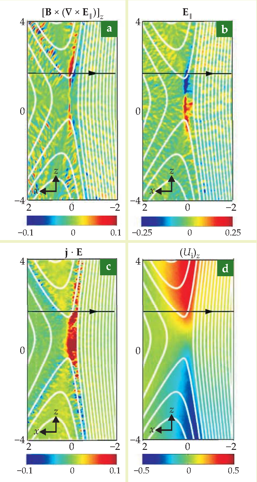
Figure 3 depicts the parallel electric fields, the electromagnetic energy conversion, and the concomitant ion acceleration due to reconnection.

Satellite measurements

On 2 April 2001, NASA’s Polar satellite crossed a reconnecting magnetopause north of the reconnection site along a trajectory illustrated by the horizontal line across each panel of figure 3. The crossing, whose data are shown in figure 4, occurred at an altitude of 52 240 km.

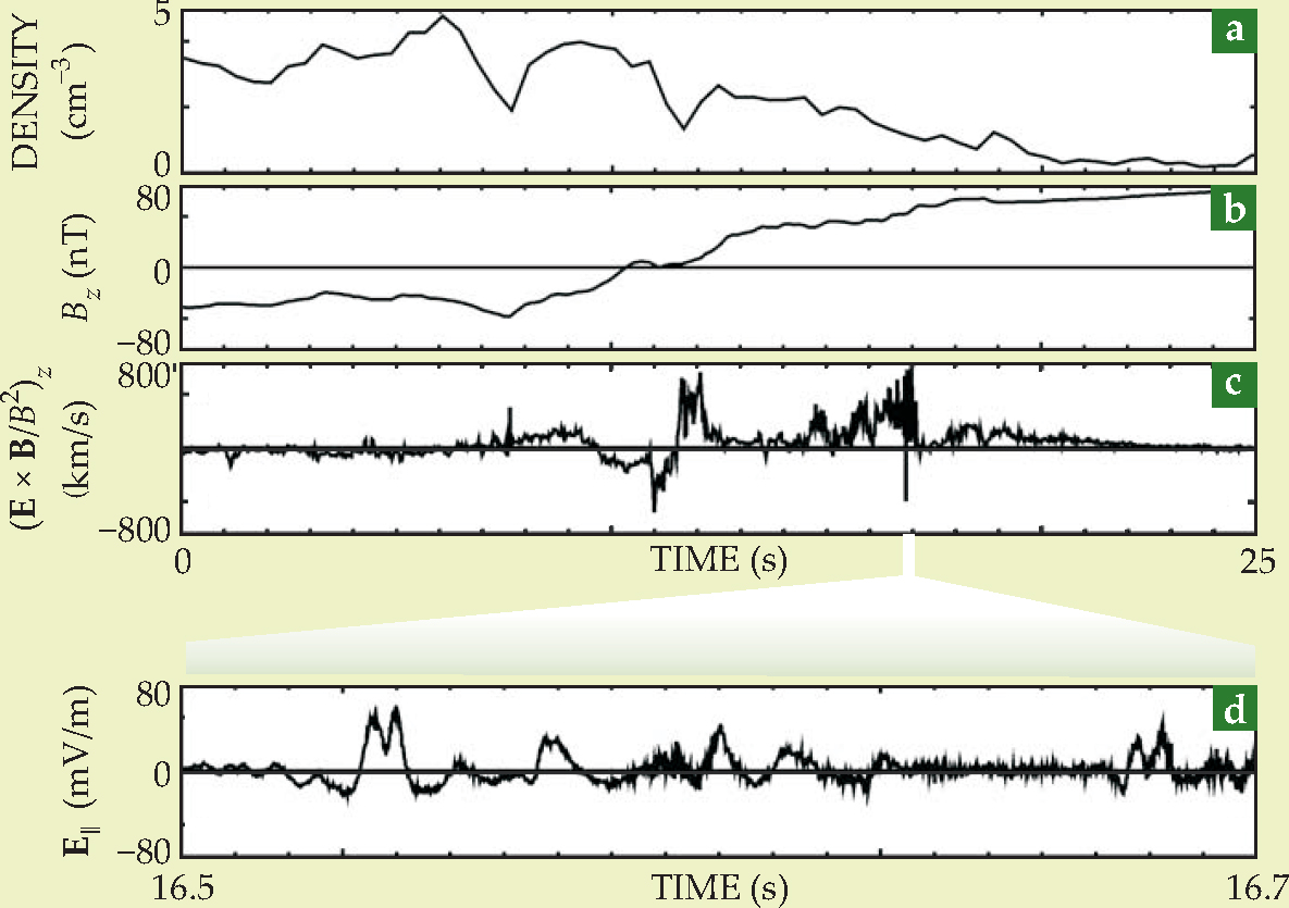
An interesting feature seen in both computer simulations and space measurements is the presence of parallel electric fields on the magnetosphere side, well away from thereconnection site itself. The fields are an order of magnitude larger than calculated in the simulations. Understanding that discrepancy is at the forefront of current research.

Energy conversion

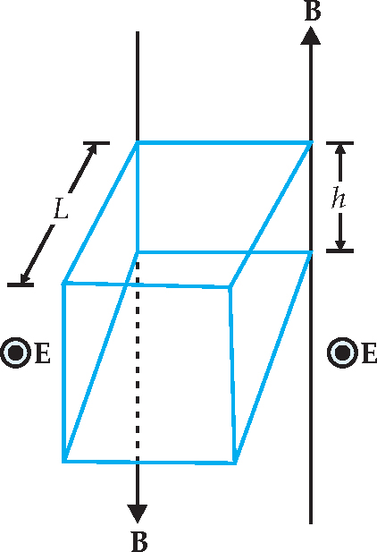
The energy available per cold particle in a single reconnection event is on the order of $\raisebox{1ex}{$1$}\!\left/ \!\raisebox{-1ex}{$2$}\right.$ mV _A ², where V _A is the Alfvén speed (B ²/µ_o nm) ^{$\raisebox{1ex}{$1$}\!\left/ \!\raisebox{-1ex}{$2$}\right.$} , with µ_o the permeability of free space (see figure 5). The outflow energy for an electron, $\raisebox{1ex}{$1$}\!\left/ \!\raisebox{-1ex}{$2$}\right.$ m _e V _A ², is then about 1 eV, many orders of magnitude less than the energies of electrons observed in the magnetosphere or in solar flares.

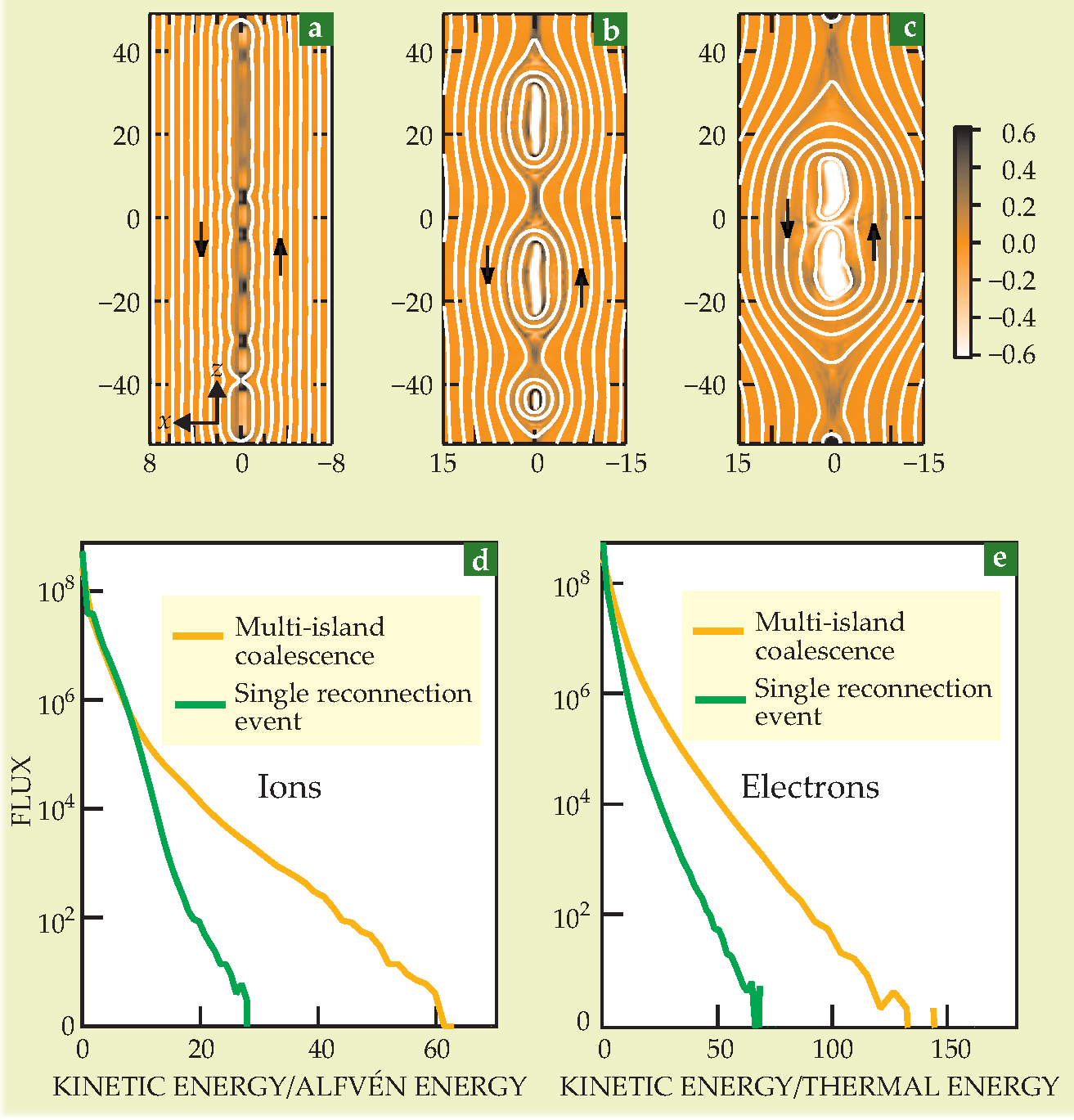
Because the bulk particle energy gained in a single reconnection event is insufficient to explain observations, how can reconnection be associated with the rapid acceleration of electrons to high energies in space? According to PIC simulations, reconnection at more than one site along a current sheet can produce magnetic islands as a result of two separate reconnection outflow regions that coalesce. The conversion of the electromagnetic energy to particle energy in those islands can then give rise to high energy tails extending to a few hundred times the electron thermal energy. Examples of ion and electron spectra shown in figure 6 from a PIC simulation—using an m/m _e ratio of 25—illustrate the energy gain from island formation.

The situation is more complex for solar flares. In that case, observations indicate that as much as 50% of the released energy appears in the form of energetic electrons. One recent suggestion ¹⁰ is that multiple reconnection sites may be involved: In three dimensions with magnetic field lines intertwined like spaghetti, many regions of sheared magnetic fields will appear; reconnection can thus occur at many locations simultaneously, and magnetic islands may be volume filling rather than constrained to form as a single chain along the symmetry line of a current sheet. Those islands might then grow and contract, and electrons would gain energy by reflecting from the contracting islands, as in the classic Fermiacceleration mechanism. The repetitive interaction of electrons with many such islands may allow large numbers of electrons to be accelerated to high energies.

Future directions

In this article we’ve discussed magnetic reconnection from a first-principles perspective based on the underlying kinetic (two-fluid) nature of a collisionless plasma. That approach is essential for understanding the small-scale physics that determines how the topology of the field lines becomes reconfigured in the vicinity of the reconnection site. However, major challenges remain in extending the kinetic approach to the macroscopic scales that characterize real systems. For example, a reconnection site in the solar corona is on the order of 10 m, much smaller than the roughly 2 × 10⁷ m typical size of x-ray bright points—coronal structures uniformly distributed over the solar surface and situated above pairs of opposite polarity magnetic fragments in the photosphere. It may never be possible to treat such large-scale structures using a first-principles approach, so reduced physics models such as MHD are likely to remain necessary to address the macroscopic consequences of reconnection.

Even within the kinetic framework, fundamental issues are yet to be resolved. Our picture of reconnection is largely based on 2D models in which no variation in the direction of the initial current is considered. One can then speak of a single reconnection site. But when one drops the 2D restriction, a new class of current-aligned instabilities becomes possible. ¹¹ Such instabilities could give rise to additional sources of dissipation that modify the reconnection rate.

Alternatively, the instabilities might alter the spatial structure of the current layer, which could, in turn, result in multiple reconnection sites that form and interact with each other. Results of 3D PIC simulations for electron-positron pair plasmas indicate that the reconnection onset is patchy and occurs at multiple sites that self-organize into a single, large diffusion region. ¹² That region tends to elongate in the direction of outflowing particles and becomes unstable to the formation of structures with finite extent in the current direction. As the capabilities of massively parallel supercomputers continue to increase, 3D PIC simulations of reconnection will become widespread.

Although numerical studies have been invaluable to our understanding of magnetic reconnection, hypotheses must ultimately be tested against observations. NASA is developing an ambitious four-spacecraft mission—Magnetospheric Multiscale, whose launch is scheduled for 2014—to probe the microphysics responsible for magnetic reconnection in the boundary regions of Earth’s magnetosphere, particularly along its dayside boundary with the solar wind and the boundary between open and closed magnetic field lines in the magnetic tail. ¹³

Magnetospheric Multiscale will also investigate how the energy conversion that occurs during magnetic reconnection accelerates particles to high energy and what role plasma turbulence plays in magnetic reconnection events. The hope is that the mission, together with its theoretical interpretation, will fundamentally advance our understanding of magnetic reconnection and the role it plays throughout the universe.

References

1. R. G. Giovanelli, Nature 158, 81 (1946). https://doi.org/10.1038/158081a0
2. J. W. Dungey, Philos. Mag. 44, 725 (1953).
3. E. G. Zweibel M. Yamada, Annu. Rev. Astron. Astrophys. 47, 291 (2009). https://doi.org/10.1146/annurev-astro-082708-101726
4. V. M. Vasyliunas, Rev. Geophys. Space Phys. 13, 303 (1975), https://doi.org/10.1029/RG013i001p00303 .
5. F. S. Mozer, J. Geophys. Res. 110, A12222 (2005), https://doi.org/10.1029/2005JA011258 .
6. L. Spitzer Jr, Physics of Fully Ionized Gases, 2nd ed., Interscience, New York (1962).
7. J. M. Dawson, Rev. Mod. Phys. 55, 403 (1983). https://doi.org/10.1103/RevModPhys.55.403
8. C. K. Birdsall, A. B. Langdon, Plasma Physics via Computer Simulation, McGraw-Hill, New York (1985).
9. P. L. Pritchett, J. Geophys. Res. 113, A06210 (2008), https://doi.org/10.1029/2007JA012930 .
10. J. F. Drake et al., Nature 443, 553 (2006). https://doi.org/10.1038/nature05116
11. J. Bu¨chner, W. S. Daughton, in Reconnection of Magnetic Fields: Magnetohydrodynamics and Collisionless Theory and Observations, J. Birn, E. R. Priest, eds., Cambridge U. Press, New York (2007), pp. 144–53.
12. L. Yin et al., Phys. Rev. Lett. 101, 125001 (2008). https://doi.org/10.1103/PhysRevLett.101.125001
13. J. L. Burch J. F. Drake, Amer. Sci. 97, 392 (2009). See also the Magnetospheric Multiscale mission website at http://mms.space.swri.edu/index.html . https://doi.org/10.1511/2009.80.392
14. F. S. Mozer P. L. Pritchett, J. Geophys. Res. 115, A04220 (2010), https://doi.org/10.1029/2009JA014718 .
More about the authors
Forrest Mozer is a professor with the space physics group at the University of California, Berkeley, and Philip Pritchett is a research physicist at the University of California, Los Angeles.
Forrest S. Mozer, 1 University of California, Berkeley, US .
Philip L. Pritchett, 2 University of California, Los Angeles, US .