Introducing groundwater physics
DOI: 10.1063/1.2743123
Water is critical to the survival of life and the continued existence of the natural environment on Earth. Most people visualize rivers and lakes as the water resources in need of protection, but groundwater makes up more than 98% of available freshwater resources, supplies 40% of the drinking water in the US and 70% in China, and is the main source of domestic water supply in most European countries. Groundwater provides approximately one-fifth of the world’s industrial, agricultural, and municipal water. The science of groundwater hydrology, a discipline of geoscience, forms the framework in which management decisions about groundwater resources are made. Groundwater hydrologists are concerned with the development of groundwater for municipal, industrial, and agricultural uses; remediation of resources affected by contamination; and protection of resources from future contamination. Scientifically, the field of groundwater hydrology is diverse and includes specializations in groundwater–surface water interaction, ecohydrology, hydrogeochemistry, hydrogeomicrobiology, contaminant hydrogeology, groundwater modeling, and hydrogeophysics. 1
This article, intended as an introduction to some of the physics important in groundwater hydrology, cannot possibly capture all aspects of such a broad and complex discipline. Specialists in groundwater hydrology will disagree with any particular choice of topics and emphasis; this article provides just one view of some of the physics of quantitative groundwater hydrology.
Some definitions
Groundwater hydrology is the study of water in the subsurface. Such water is found in the void space in porous materials such as sand and sandstone, in fine-grained materials such as silt and clay, and in the fractures of limestone and crystalline rock such as granite. Subsurface water, as shown in figure 1, is found in the unsaturated zone above the water table, where some of the void space is filled with water and some with air, and in the saturated zone below the water table, where all the void space is filled with water. Traditionally and in this article, the term groundwater refers only to water in the saturated zone below the water table where water flows freely into wells under pore pressure greater than atmospheric pressure.

Figure 1. Subsurface water in the unsaturated zone above the water table and in the saturated zone below the water table. Only the water in the saturated zone is considered groundwater.
(Adapted from the US Geological Survey.)
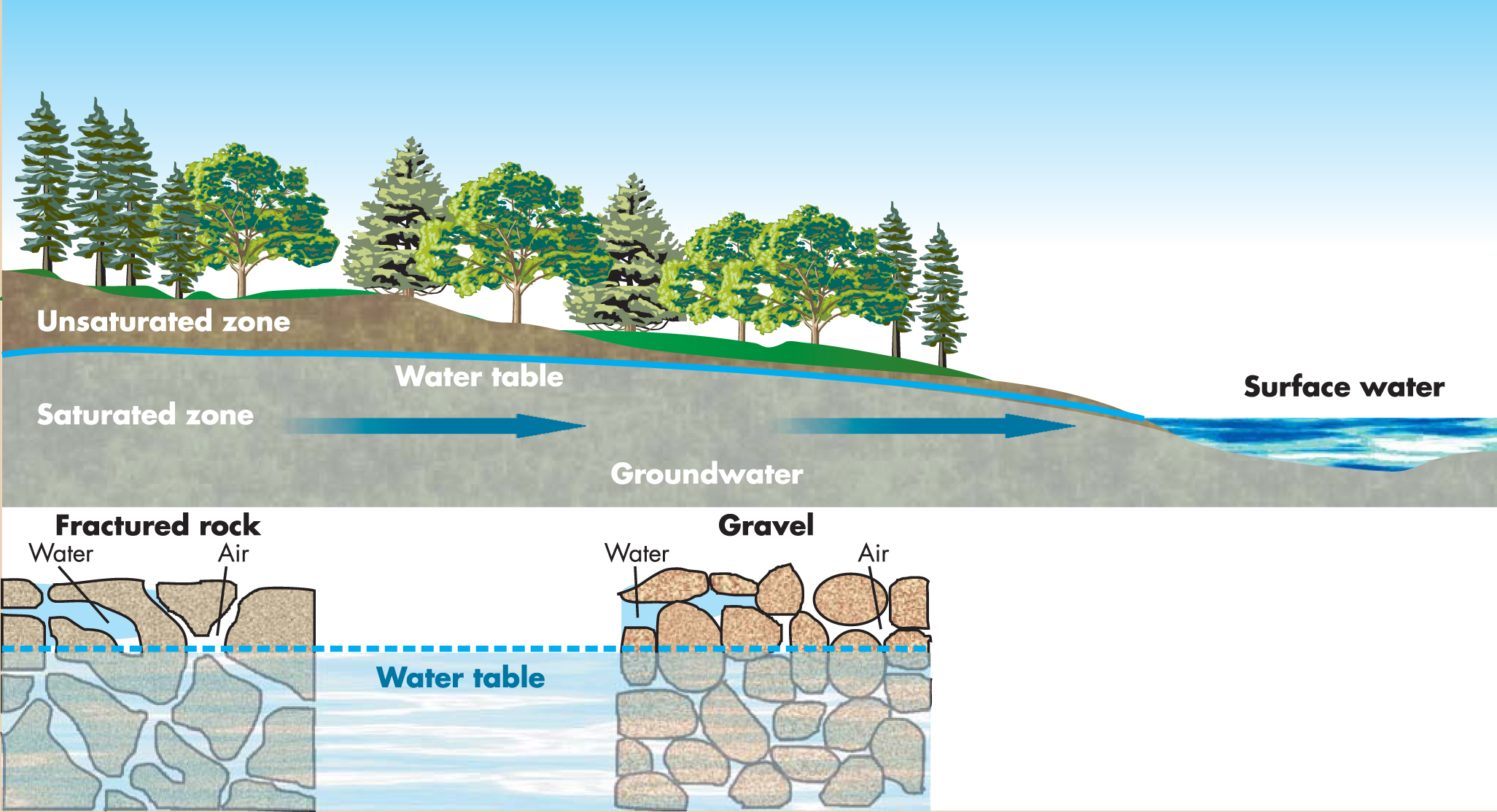
An aquifer, the primary type of groundwater reservoir, is a body of porous material, either consolidated rock or unconsolidated material such as sand and gravel, that yields significant quantities of water to wells and springs. The definition restricts aquifers to fully saturated material, but otherwise it is vague and unsatisfactory because the amount of water that is considered significant is subjective. For example, a particular geological body of porous material could be an aquifer for domestic water use but not for high-capacity industrial use.
Fundamental laws
In 1856, Henry Darcy published a lengthy report entitled Les Fontaines Publiques de la Ville de Dijon. In one of the eight appendices, he presented an equation inferred from the results of his experiments on 2.5-meter-long sand columns. The publication of that equation, now called Darcy’s law, marks the beginning of groundwater hydrology as a quantitative science, although there were some earlier observations of groundwater flow. 2
Darcy’s law, which describes the flow of groundwater through a porous material, is mathematically similar to Fourier’s, Ohm’s, and Fick’s laws, which describe thermal conduction, electrical conduction, and diffusion of a solute. All four laws, shown in the
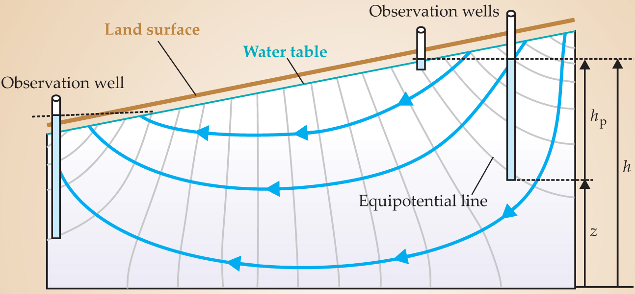
The Darcy’s-law analogue of temperature, electrical potential, and solute concentration is head h, a measure of the potential energy of groundwater. The potential energy per unit mass of groundwater is generally equal to gh, where g is the acceleration due to gravity. Head is the sum of elevation head z, which is a measure of gravitational potential energy, and pressure head h p, which is a measure of potential energy due to pore pressure. Head is measured in the field as the elevation to which the water level rises in an observation well; a three-dimensional array of heads defines a potential field and determines the direction of groundwater flow, as shown in figure 2. Darcy recognized that water flows from higher to lower head, but the realization that head is a potential was not articulated until 1940, when the geophysicist M. King Hubbert published a classic paper on the theory of groundwater flow. Then in 1956 Hubbert showed that Darcy’s law can be derived as a special case of the Navier–Stokes equations. 3

Figure 2. Delineation of groundwater flow using observation wells to determine head h, a measure of the potential energy of groundwater. Total head is equal to elevation head z plus pressure head h p. Equipotential lines connect points of equal head. In a homogeneous, isotropic medium, flow lines are drawn perpendicular to the equipotential lines with water flowing from higher to lower head. When the head in the well is above land surface—for example, at the well shown at the left-hand side of the figure—the well is said to be a flowing well because water would flow out at the surface if not confined by a well pipe.
The rate at which water flows through a porous medium is governed by the hydraulic conductivity K. Whereas the analogous parameters thermal conductivity, electrical conductivity, and the diffusion coefficient are often treated as scalars, hydraulic conductivity is a symmetric tensor, which allows for anisotropy in the porous material. Hydraulic conductivity depends on the viscosity and density of water and on the properties of the porous medium; the permeability k is a related parameter that describes the transmission properties of the medium independently of the fluid. Some methods for measuring hydraulic conductivity are described in
Not only are Fourier’s, Ohm’s, and Fick’s laws mathematically analogous to Darcy’s law, but each is also important in solving groundwater problems. Ohm’s law is not directly relevant to the physics of groundwater flow, but has applications in geophysical methods for site characterization: Workers use resistivity and electromagnetic surveys to infer subsurface characteristics, especially the presence of contaminated water. Darcy’s, Fick’s, and Fourier’s laws, together with the principle of conservation of mass, enable the derivation of governing equations, presented in
Groundwater flow
When Darcy’s law is applied at a macroscopic scale, the Darcy flux q averages variations in velocity that occur as water flows in nonlinear (tortuous) paths determined by the pore space within the porous material. Although tortuosity can be quantified experimentally using the formation factor in Archie’s law 4 (see the article by Po-zen Wong, Physics Today, December 1988, page 24 ), in practice the effects of tortuosity are lumped into the permeability.
The linear relation between head gradient and flux given by Darcy’s law is valid for most velocities that occur in natural groundwater systems, but it breaks down at high velocities. In granular porous material, the breakdown occurs at a Reynolds number between 1 and 10. At those Reynolds numbers, flow is still laminar; the transition to turbulent flow occurs at Reynolds numbers above 100. 3,4 Few measurements of flow have been made at low velocities, corresponding to Reynolds numbers less than 0.01, which occur in porous material of very low permeability, so the applicability of Darcy’s law at such velocities remains an untested hypothesis. 5
Although Darcy’s law is valid under transient conditions, transient analysis requires a storage parameter, called the specific storage, to quantify the rate of uptake and release of water to and from storage within the pore space or in fractures of the porous medium. Discovery of the physics of storage and development of a mathematical formulation for the storage term occurred over an extended period of time, mainly during 1928–69, with researchers drawing from soil mechanics and poroelastic theory.
6
Water is released from storage when the water table falls and is taken up into storage when the water table rises. Water is also released from storage by compression of the porous material, when water is pumped out of an aquifer, which causes the land surface to subside. Compression of an aquifer may also occur in response to external forces on the land surface, as described in
In its simplest form, the governing equation for groundwater flow reduces to the Laplace equation, which represents flow in a homogeneous, isotropic aquifer under steady-state conditions. That the Laplace equation could be used to solve for groundwater flow was recognized relatively soon after the publication of Darcy’s law, but it wasn’t until much later that mathematical models were generally applied in groundwater hydrology.
| Darcy's law | Fourier's law | Fick's law | Ohm's law | |
|---|---|---|---|---|
| Flux of | Groundwater, q (m/s) | Heat, q H (W/m2) | Solute, f (g/m2·s) | Charge, i (A/m2) |
| Potential | Head, h (m) | Temperature, T (K) | Concentration, C (g/m3) | Voltage, V (V) |
| Medium property | Hydraulic conductivity, K (m/s) | Thermal conductivity, κ (W/K·m) | Diffusion coefficient, D d (m2/s) | Electrical conductivity, σ (1/Ω·m) |
| q = −K ∇h | q H = −κ ∇T | f = −D d ∇C | i = −σ ∇V |
Flux of |
Groundwater, q (m/s) |
Heat, q H (W/m2) |
Solute, f (g/m2·s) |
Charge, i (A/m2) |
Potential |
Head, h (m) |
Temperature, T (K) |
Concentration, C (g/m3) |
Voltage, V (V) |
Medium property |
Hydraulic conductivity, K (m/s) |
Thermal conductivity, κ (W/K·m) |
Diffusion coefficient, D d (m2/s) |
Electrical conductivity, σ (1/Ω·m) |
q = −K ∇h |
q H = −κ ∇T |
f = −D d ∇C |
i = −σ ∇V |
The door to mathematical modeling of groundwater flow was opened in 1935 by Charles V. Theis, who adapted an analytical solution from the heat-flow literature to describe transient groundwater flow to a pumping well. 7 Theis’s work revolutionized groundwater hydrology and led to an outpouring of papers by other researchers on analytical solutions to describe flow to wells under a variety of hydraulic conditions.
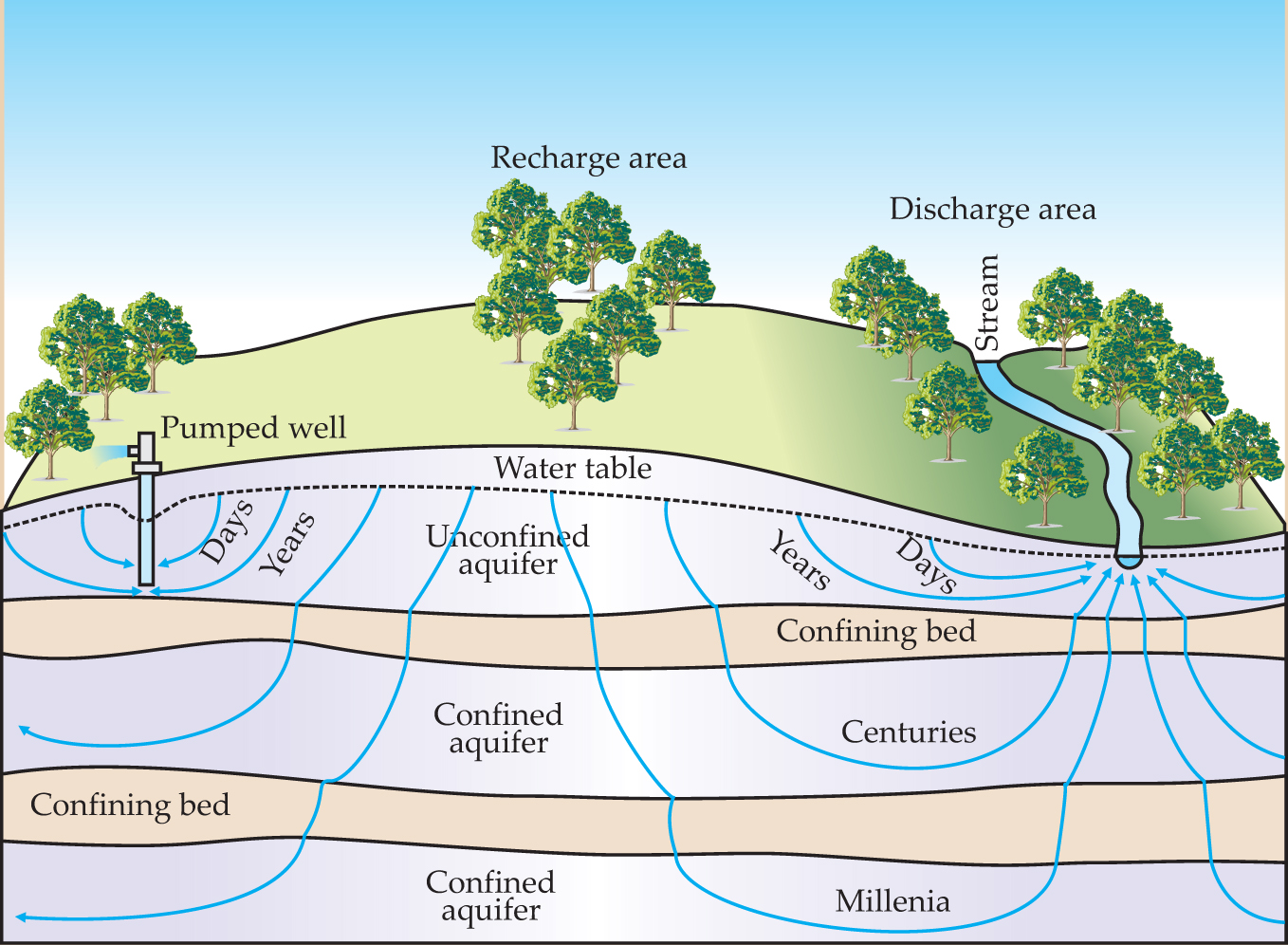
In the 1960s attention turned toward quantifying and understanding regional flow systems and the interaction of groundwater with rivers, lakes, wetlands, and the ocean, as exemplified in figure 3. The interaction of groundwater with surface water is an area of practical interest and active research. 8 For many lakes, groundwater discharge is an important source of water and nutrients; groundwater discharge to oceans is a significant source of nutrients in coastal and estuarine environments. Mixing of groundwater and river water in the so-called hyporheic zone beneath a stream allows a host of unique macroorganisms to thrive in that interface area. Groundwater hydrologists have investigated many other types of phenomena, including flow in low-permeability media 5,9 that are potential sites for disposal of radioactive waste.

Figure 3. Regional groundwater flow. Flow lines in a regional flow system composed of aquifers and less permeable confining beds. Water infiltrates the water table in the recharge area and leaves the system and enters a stream in the discharge area. Time scales of ground-water flow and drawdown in the water table around a pumped well are also shown.
(Adapted from T. C. Winter et al.,
Estimating hydraulic conductivity
Hydraulic conductivity K, the fundamental parameter that describes the transmission of water through a porous medium, varies over 13 orders of magnitude from 10−14 m/s for unfractured crystalline rock to 10−1 m/s for gravel. It can be measured in a laboratory by flowing water at a constant rate through a column packed with porous material. Then K can be calculated from Darcy’s law. However, the small sample of material in laboratory columns is not representative of the heterogeneous mixture of material in an aquifer.
Charles V. Theis devised a transient mathematical model for estimating not only an average hydraulic conductivity under field conditions but also a value for the storage parameter. 7 In Theis’s method, illustrated in the figure, a well is pumped at a specified rate Q, and the decline of the water level (drawdown) is measured in one or more observation wells. The pumping well and the observation wells are open to the aquifer. Then drawdown in the potentiometric surface, as shown in the figure (or the drawdown in the water table as shown in figure 3), is used to calculate hydraulic conductivity.
When it is not possible to perform a pumping test, K can be estimated using measurements made in the observation well itself. A cylindrical object called a slug is dropped into the well to displace the water. Then the slug is quickly removed and the recovery in water level is measured; K and the storage parameter are calculated based on the recovery curve. So-called slug tests are widely used in groundwater practice.
Pumping tests give average values of K within the area affected by pumping. Slug tests give values of K close to the well. Hydraulic tomography and push–pull tests 18 can be used to obtain finer resolution of the spatial variability in K. During hydraulic tomography, pumping tests are performed at multiple positions in three-dimensional space by means of a network of wells. Each well is open to the aquifer at several vertical positions. The discrete vertical interval being pumped is isolated, and drawdown is measured in the other vertical intervals as well as in the rest of the network. The drawdown measurements from all the wells are analyzed simultaneously to determine a 3D array of hydraulic conductivity values to produce a kind of computed tomography (CT) scan of the aquifer. In a push–pull test, multilevel boreholes are installed and slug tests are performed at each level in each borehole, again producing a 3D array of hydraulic conductivity values. (Figure adapted from G. M. Hornberger et al., Elements of Physical Hydrology , Johns Hopkins U. Press, Baltimore, MD, 1998.)

Governing equations
The governing equation for groundwater flow is derived by combining Darcy’s law (see the
where q is the flux of groundwater, t is time, head h is a measure of the potential energy of groundwater, the specific storativity Ss is the volume of water removed from storage per unit volume of porous material in response to a decline in head, and W represents a sink or source of water, such as recharge from precipitation or pumping from a well. The combined equation is
The coordinate system is usually chosen so that the off-diagonal components of the symmetric tensor K are zero, and equation
A similar combination of Fourier’s law and a heat-balance equation gives the governing equation for heat flow in groundwater:
where T is temperature, ρw and c w are the density and specific heat of water, ρ and c are the density and specific heat of the rock–water matrix, and κe is a term that includes the effective thermal conductivity of the rock–water matrix. Specifically,
where κo = θκw + (1 − θ)κg. The porosity θ is the fraction of the total volume that is occupied by water, α* is the thermal dispersivity, and κw and κg are the thermal conductivities of water and of the rock. The thermal conductivities of porous materials range from 0.2 W/K·m for dry sediments to 4.5 W/K·m for sandstone, and the thermal conductivity of water is 0.6 W/K·m. Thus, the range in thermal conductivity is much smaller than the range in hydraulic conductivity. Equations 2 and 4 are coupled through the hydraulic conductivity, which is temperature dependent, and the water flux.
A form of Fick’s law and a mass-balance equation yield the governing equation for transport of a solute in groundwater:
where Ck is the concentration of species k, D is the dispersion tensor, qsCs k is the rate at which solute is introduced through a source or removed through a sink, and Σ Rn represents the addition or removal of solute due to chemical reaction. Equations 2 and 6 are coupled through the water flux q.
Computer codes can solve for groundwater flow alone or groundwater flow coupled to heat flow and solute transport.
Heat flow
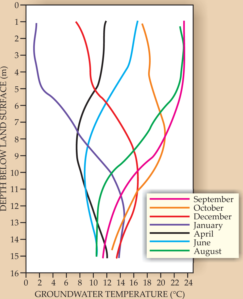
Researchers recognized in the early 19th century that temperature measurements could be used to trace groundwater movement, since seasonal changes in the temperature of surface water are reflected in the groundwater temperature, as shown in figure 4. Current interest in using heat as a tracer is motivated in part by the development of new technologies, such as fiber-optic cables, for measuring temperatures in surface and subsurface water. 10

Figure 4. Temperature profiles showing seasonal fluctuations beneath the Rio Grande in central New Mexico. Temperature was measured at 15-cm intervals using a probe equipped with a thermistor. An annual temperature envelope can be fitted to the suite of profiles and used with a solution of the heat transport equation to estimate vertical groundwater velocity beneath the stream.
(Adapted from J. R. Bartolino, in
The governing equation for heat flow combines Fourier’s law with conservation of energy and includes a term for advection of heat by flowing groundwater. The heat-transport equation, shown in
Compressible aquifers
In 1928 Oscar E. Meinzer, one of the founding fathers of groundwater hydrology, clearly articulated the concept of a compressible aquifer in which water is squeezed out of the pore space in a porous medium in response to pumping. 6 In 1939 Charles Jacob described how the external loading from a train stopping at a station near an observation well produced a temporary aquifer compression that caused a rise in water level as water was squeezed out of the pore space into the well.
Furthermore, changes in atmospheric pressure affect water levels in wells in confined aquifers, and water levels are affected by Earth tides and by tidal fluctuations in the ocean, lakes, and streams. Seismic waves induced by earthquakes also cause changes in stress and pore pressure that cause changes in water levels in wells. (Figure adapted from J. G. Ferris et al., US Geological Survey Water-Supply paper 1536-E, 1962.)

Solute transport
Fick’s law describes diffusion of solutes from higher to lower concentrations. In groundwater-flow systems, however, mixing by diffusion within pore spaces and fractures is a relatively minor effect except in media of very low permeability. Much more significant mixing occurs as solutes move by advection along the tortuous flow paths defined by the network of pores and fractures.
To retain Darcy’s law to describe flux of groundwater and simultaneously quantify solute transport in porous material, a “fudge factor” known as dispersivity is introduced to account for mixing (dispersion) caused by tortuosity. A dispersion tensor D is defined as the sum of the effective diffusion coefficient and a term for dispersion, which is expressed as a product of the average linear velocity and a mixing length or dispersivity factor, representing deviations from the average linear velocity given by Darcy’s law. Following G. I. Taylor, who analyzed longitudinal dispersion in pipe flow where the dispersion is proportional to the square of the velocity 12 (see the article by Michael Brenner and Howard Stone, Physics Today, May 2000, page 30 ), groundwater hydrologiste describe the mixing process by a Fickian law in which the dispersion tensor replaces the diffusion coefficient of Fick’s law.
The situation is more complicated at the larger length scale characteristic of field measurements, where mixing occurs because of variations in velocity due to differences in the hydraulic conductivities of porous media such as sand, silt, and clay in alluvial deposits. The large-scale mixing or dispersion caused by such heterogeneities can be represented directly if each heterogeneity is explicitly included in the model, but mapping the hydraulic conductivity at the scale and level of detail required is usually impossible. When heterogeneities are not explicitly represented in detail, the dis-persivities in the dispersion tensor are effectively a measure of the dimensions of the unmodeled heterogeneities present in the flow field. Such dispersivity values may range up to hundreds of meters 12 in contrast to the dispersivities on the order of 1 meter or less that are sufficient to represent mixing in laboratory columns filled with relatively homogeneous porous material.
An immense body of literature is devoted to efforts at quantifying dispersivities and the dispersion process in heterogeneous groundwater systems, but there is still no consensus on how to derive field-scale dispersivity values from information about hydraulic conductivity. Some researchers advocate using geostatistical models to simulate many possible realizations of heterogeneities at the field scale.
Other aspects of the contaminant-transport problem are concerned with representation of variable-density fluids— for example, fresh and salt water in coastal aquifers, and dense and light nonaqueous-phase liquids—and chemical reactions. 13 Reactive transport in groundwater is important in engineering approaches to prevent aquifer contamination and to remediate contaminated aquifers (see the article by David Clark, David Janecky, and Leonard Lane, Physics Today, September 2006, page 34 ).
Future challenges
This article has touched on only a few aspects of the basic physics of groundwater hydrology, a diverse and complex field concerned with both practical problems and fundamental scientific questions. The future of groundwater hydrology was discussed recently in a special issue of the Hydrogeology Journal. 14 One point of debate is whether the field is mature with most of the basic issues resolved, or whether many more fundamental questions remain. 15 Certainly, the basic physics of groundwater flow and transport of heat and solutes in the subsurface is understood, yet some details of those processes remain unclear. Analytical and numerical solutions to the governing equations are available, and new analytical and improved numerical solutions continue to be developed for new and more complex problems. Moreover, the novel application of traditional tools to problems in emerging areas such as ecohydrology, geomicrobiology, marine hydrogeology, and extraterrestrial hydrogeology will uncover new and perhaps fundamental questions about groundwater processes. Newer tools involving isotopes and remote sensing 16 such as the satellite-based imaging technique InSAR (described by Matt Pritchard, Physics Today, July 2006, page 68 ) will facilitate the study of groundwater processes in new ways and will likely generate new questions.
Furthermore, the difficulty in quantifying the complexity inherent in natural systems is a fundamental unresolved issue confronting all of groundwater hydrology. Although the physics used in groundwater hydrology is well understood and proven to work for simple geological systems, the challenge lies in applying the known equations to complex real-world systems whose structures and external conditions are not fully known. A critical unresolved question is whether it is possible to determine in detail the large-scale permeability structure of an aquifer from small-scale measurements in wells. In site-specific field applications, values of other system parameters such as porosity, recharge rate, thermal conductivity, and chemical reaction rates and processes are also difficult to quantify. In short, models of groundwater systems are inherently plagued by uncertainty. According to Clifford Voss, 14 groundwater hydrology “is not well suited to quantitative prediction and is best suited to providing hydrogeologists with theoretical and science-based intuition that they can apply when suggesting solutions to complex practical problems.” Tools such as inverse methods 14,17 and stochastic simulation 14 are available to help address the uncertainty problem arising from incomplete system characterization, but dealing with uncertainty is still a formidable challenge for the future.
References
1. The following are a selection of textbooks on various aspects of groundwater hydrology: J. B. Jones, P. J. Mulholland, eds., Streams and Ground Waters, Academic Press, San Diego, CA (2000);
M. P. Anderson, W. W. Woessner, Applied Groundwater Modeling: Simulation of Flow and Advective Transport, Academic Press, San Diego, CA (1992);
C. W. Fetter, Contaminant Hydrogeology, 2nd ed., Macmillan, New York (1999);
F. H. Chapelle, Ground-Water Microbiology and Geochemistry, 2nd ed., Wiley, New York (2001);
C. Zheng, G. D. Bennett, Applied Contaminant Transport Modeling, 2nd ed., Wiley InterScience, Hoboken, NJ (2002);
Y. Rubin, S. S. Hubbard, eds., Hydrogeophysics, Springer, New York (2005). https://doi.org/10.1007/1-4020-3102-5
C. R. Fitts, Groundwater Science, Academic Press, San Diego, CA (2002) is a general textbook, but there are many others.2. C. W. Fetter Jr, Ground Water 42, 790 (2004). https://doi.org/10.1111/j.1745-6584.2004.tb02734.x
3. M. K. Hubbert, J. Geol. 48, 785 (1940); https://doi.org/10.1086/624930
Pet. Trans. AIME 207, 222 (1956);
W. G. Gray, C. T. Miller, Adv. Water Resour. 29, 1745 (2006). https://doi.org/10.1016/j.advwatres.2006.03.0104. R. E. Chapman, Geology and Water: An Introduction to Fluid Mechanics for Geologists, Martimus Nijhoff, the Hague, the Netherlands (1981), p. 55.
5. C. E. Neuzil, Water Resour. Res. 22, 1163 (1986). https://doi.org/10.1029/WR022i008p01163
6. H. F. Wang, Theory of Linear Poroelasticity with Applications to Geomechanics and Hydrogeology, Princeton U. Press, Princeton, NJ (2000);
T. N. Narasimhan, Ground Water 44, 488 (2006); https://doi.org/10.1111/j.1745-6584.2006.00160.x
O. E. Meinzer, Econ. Geol. 23, 263 (1928). https://doi.org/10.2113/gsecongeo.23.3.2637. C. V. Theis, Trans. Am. Geophys. Union 16, 519 (1935). https://doi.org/10.1029/TR016i002p00519
8. T. C. Winter, Hydrogeol. J. 7, 28 (1999); https://doi.org/10.1007/s100400050178
F. Klijn, J.-P. M. Witte, Hydrogeol. J. 7, 65 (1999); https://doi.org/10.1007/s100400050180
M. Hayashi, D. O. Rosenberry, Ground Water 40, 309 (2002); https://doi.org/10.1111/j.1745-6584.2002.tb02659.x
P. J. Hancock, A. J. Boulton, W. F. Humphreys, Hydrogeol. J. 13, 98 (2005). https://doi.org/10.1007/s10040-004-0421-69. S. P. Neuman, Hydrogeol. J. 13, 124 (2005); https://doi.org/10.1007/s10040-004-0397-2
M. Bakalowicz, Hydrogeol. J. 13, 148 (2005); https://doi.org/10.1007/s10040-004-0402-9
V. Remenda, Hydrogeol. J. 9, 3 (2001). https://doi.org/10.1007/s10040000011610. J. Selker et al., Geophys. Res. Lett. 33, L24401 (2006). https://doi.org/10.1029/2006GL027979
11. M. P. Anderson, Ground Water 43, 951 (2005). https://doi.org/10.1111/j.1745-6584.2005.00052.x
12. G. I. Taylor, Proc. R. Soc. London, Ser. A 219, 186 (1953); https://doi.org/10.1098/rspa.1953.0139
R. L. Detwiler, H. Rajaram, R. J. Glass, Water Resour. Res. 36, 1611 (2000); https://doi.org/10.1029/2000WR900036
D. Schulze-Makuch, Ground Water 43, 443 (2005); https://doi.org/10.1111/j.1745-6584.2005.0051.x
G. Dagan, Annu. Rev. Fluid Mech. 19, 183 (1987). https://doi.org/10.1146/annurev.fl.19.010187.00115113. R. W. Ritzi Jr, Z. Dai, Geosphere 2, 73 (2006); https://doi.org/10.1130/GES0202INT.1.
C. T. Simmons, Hydrogeol. J. 13, 116 (2005). https://doi.org/10.1007/s10040-004-0408-314. Special issue, “The Future of Hydrogeology,” Hydrogeol. J. 13 (March 2005).
15. F. W. Schwartz, M. Ibaraki, Ground Water 39, 492 (2001); https://doi.org/10.1111/j.1745-6584.2001.tb02337.x
F. W. Schwartz, M. Ibaraki, Ground Water 40, 317 (2002); https://doi.org/10.1111/j.1745-6584.2002.tb02660.x
F. M. Phillips, Ground Water 40, 217 (2002); https://doi.org/10.1111/j.1745-6584.2002.tb02647.x
C. T. Miller, W. G. Gray, Ground Water 40, 224 (2002) https://doi.org/10.1111/j.1745-6584.2002.tb02650.x
C. -F. Tsang, Ground Water 43, 296 (2005). https://doi.org/10.1111/j.1745-6584.2005.0023.x16. C. Kendall, J. J. McDonnell, eds., Isotope Tracers in Catchment Hydrology, Elsevier, New York (1998);
D. L. Galloway, J. Hoffmann, Hydrogeol. J. 15, 133 (2007). https://doi.org/10.1007/s10040-006-0121-517. M. C. Hill, C. R. Tiedeman, Effective Groundwater Model Calibration, with Analysis of Data, Sensitivities, Predictions, and Uncertainty, Wiley InterScience, Hoboken, NJ (2007).
18. T. -C. Jim Yeh, C. -H. Lee, Ground Water 45, 116 (2007); https://doi.org/10.1111/j.1745-6584.2006.00292.x
S. M. Sellwood, J. M. Healey, S. Birk, J. J. Butler Jr, Ground Water 43, 19 (2005). https://doi.org/10.1111/j.1745-6584.2005.tb02282.x
More about the authors
Mary Anderson is a professor of geology and geophysics at the University of Wisconsin–Madison.
Mary P. Anderson, 1 University of Wisconsin–Madison, US .


