Getting a grip on the electrical grid

Expected to reliably deliver power whenever and wherever consumers demand it, today’s electrical grids are the largest engineered systems ever built. In recent years these seemingly mundane collections of wires and generators have become the focus of heated societal discussions as the grids of tomorrow are designed and debated. The topics of those discussions are quite interdisciplinary and range from the analysis of large-scale blackouts ¹ to controls for renewable-energy integration and smart utilization of appliances. ² The debate is understandable because the systems affect almost every aspect of our day-to-day lives.

Today’s grids already exhibit complex nonlinear dynamics; for example, the collective effects of thousands of induction motors found in air conditioners and other small consumer appliances may produce serious malfunctions of sections of grid. Such collective dynamics are not well understood and are likely to become more complex as consumer appliances become more intelligent and autonomous. Today’s grids have evolved to be resilient only against simple perturbations like the sudden loss of a generator. Tomorrow’s will have to integrate the intermittent power from wind and solar farms whose fluctuating outputs create far more complex perturbations. Guarding against the worst of those perturbations will require taking protective measures based on ideas from probability and statistical physics.

However, before tomorrow’s grids can be engineered, and even before many of the phenomena in today’s grids can be effectively controlled, scientists and engineers must first understand the grid’s behavior over a broad spatiotemporal scale—from milliseconds to hours and from tens of meters to thousands of kilometers. In this article we outline the physics and phenomena associated with grid behavior. For a broader treatment of control and optimization of the grid, interested readers can turn to the recent literature. ^{2 , 3}

Grid physics

Basic physics largely determined the early evolution of electrical power systems. Nikola Tesla’s alternating-current designs were favored over Thomas Edison’s direct current because the materials and technology available more than a century ago enabled easier transformation of AC power between relatively low voltage, at which it is generated and consumed, and high voltage, which allows for low-loss, long-distance power transmission. Electrification proceeded with small, single-generator town- or county-sized power systems merging to create more reliable multigenerator networks.

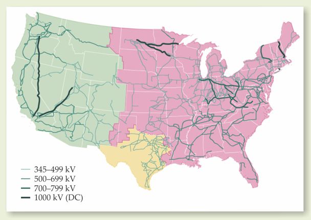
That bottom-up evolution led to regionally strong grids with weaker links to neighboring regions—a structure that affects the stability, reliability, control, and economics of today’s North American grids. In the US, the evolution culminated in several major grids (see figure 1), the largest being the Eastern Interconnection, with approximately 40 000 nodes connected by some 50 000 transmission lines.

Bottom-up evolution wasn’t inevitable. Russia, which industrialized later than the US, chose to design its power system top-down, starting with an interconnected, several-thousand-kilometer-long transmission system; the smaller regional distribution systems were built and connected only after the transmission network was available. Regardless of the development path, the basic physical structure and controls are more or less the same. The creation of synchronized AC interconnections required the selection and maintenance of a single frequency. The early North American grid designers settled on 60 Hz while the Europeans chose 50 Hz. Although many personal stories about the choices exist, the reasons for them appear to be lost to history.

An electrical grid is split into two main types of networks: a large-scale transmission grid and many distribution grids, each covering a relatively smaller area. The high-voltage (100–1000 kV) power lines of the transmission grid form a highly meshed network with an average number of line connections per node of about 2.5 and a typical line length of 100 km. The transmission network is fed by power injections from centralized, roughly 500- to 5000-MW generating stations and transfers that power in turn to substations, which transform it to lower voltage, typically 10–30 kV, for delivery to customers.

Those substations have historically served as the physical and model endpoints of the transmission network. The lower-voltage distribution grids consist of many short, tree-like circuits, each a few megawatts, that extend from the substations (see the article by Clark Gellings and Kurt Yeager in Physics Today, December 2004, page 45 ).

Power and phase

Transmission and distribution grids obey the same physics. Here we lay it out in the context of the transmission grid. Power lines carry oscillating electrical current, but that current is typically associated with two types of power—real power P and reactive power Q. Real power flows when the oscillating electrical current is in phase with the oscillating voltage V = v exp(iθ) in standard phasor notation, where v is the voltage amplitude. The time-averaged flow of real power does useful work, such as turning motor shafts.

When the current is 90° out of phase with voltage, electrical energy sloshes back and forth in the transmission grid within an AC cycle. Those flows do no useful work but certainly affect the oscillating voltage throughout the grid. It is convenient to describe the oscillating power on the same footing as real power P by defining the time-averaged reactive power Q as positive when the voltage leads current by 90°.

Electrical loads consume P from the transmission grid, and they typically also consume Q. The injection and consumption of power occur at different nodes a in the grid, and transmission lines move the power from generators to loads. When all injections, loads, and line losses are in balance, the grid is in a steady state. Changes in loads and intermittent power fluctuations from renewable energy sources are mostly compensated by control systems that modify the mechanical power fed to generators. But those control systems respond slowly, over several seconds, and the fluctuating imbalances produce changes in the kinetic energy stored in the large rotational inertia I_a of individual turbine generators. The loss of kinetic energy leads to a deceleration of the generators and thus a deviation in the local grid frequency from its nominal 60 Hz.

The mathematical representation of that process is captured by the “swing equations,” an approximation of the basic power balance and grid dynamics at time scales longer than a few AC cycles: ⁴

(1) (1)

Here, (a,b) indicates the existence of an electrical line between nodes a and b, Z_ab represents its complex impedance as a sum of resistance and reactance R_ab + iX_ab, asterisks denote complex conjugation, and the local frequencies are measured as differences from the nominal frequency. The term represents the mechanical damping of frequency deviations due to control of the generators’ input power. And represents a reactive-power control that counteracts local voltage deviations; the variables and are time-relaxation parameters.

For a generator at node a, the right-hand side of equation (1) describes the balance (or imbalance) of power injections P_a and Q_a with the last term—the real and reactive power flowing away from the node through a transmission line of impedance Z_ab. In steady state, the right-hand side is zero and the grid operates at a spatially uniform frequency. But when imbalances do exist, generators interact with each other to create a complex network of coupled oscillators. This simplest representation of the physics treats only dynamics among generators. A more complete description, which includes load dynamics, can be found in the power-engineering literature. ⁴

Reliability and stability

Ideally, the transmission grid would always operate precisely at 60 Hz at a spatially constant, normalized voltage, even as its millions of consumers impose varying loads at tens of thousands of substations. But equipment failure, nonzero transmission-line impedances, and the finite response time of each generator to changing power demands mean the grid is always awash in spatial and temporal deviations about that ideal. Operators of the grid maintain its reliability by ensuring that those deviations never grow to catastrophic size while keeping the cost of electricity as low as possible.

The reliability of today’s most sophisticated transmission grids is assessed, as often as every five minutes, primarily against three criteria: so-called (N − 1) feasibility, transient stability, and voltage stability. ⁴ The first criterion verifies that a feasible steady-state power-flow solution of equation (1) exists with any one of N major components, such as a major generator or transmission line, removed from the network. Transient stability verifies, typically via the integral of equation (1), that the dynamics excited by each N − 1 event (and other plausible perturbations) actually reach the new steady state. And voltage stability gauges the robustness of the steady-state solution to changes in electrical loading, represented by P_a and Q_a in equation (1).

Although blackouts and other interruptions of service still occur, the three stability metrics serve today’s grids well. Nevertheless, grids are changing in significant ways—incorporating, for instance, time-intermittent wind and photovoltaic power in large-scale transmission grids and in consumer-scale distribution grids. The changes will lead to grids that are more stochastic and exhibit dynamics requiring new stability criteria that address emerging problems and can be evaluated faster, closer to real time.

Voltage collapse

The traditional engineering approach to modeling power systems emphasizes the quantitative behavior of individual grid devices. A physics-based approach, by contrast, attempts to capture the underlying phenomena by using the fewest number of modeling parameters required. That is the approach we outline here.

The damped dynamics of harmonic oscillators described on the left-hand side of equation (1) are driven by terms on the right, which represent a nonlinear mix of power injections and consumptions at all the nodes. The complexity of those driving terms makes it difficult to intuitively understand the dynamics. Energy function methods, ⁵ whose details are briefly outlined in the box on page 43, represent one approach to analyzing the dynamics in a way that enables a succinct and intuitive restatement of equation (1). Briefly, the grid’s state as a function of phase and voltage can be imagined as moving along the contours of a high-dimensional potential energy landscape E(θ, v).

Figure 2 shows two such energy landscapes, each with a constant P and constant Q load connected to a constant-voltage node through a single inductive transmission line. In the lightly loaded case (left) there exists a local minimum energy at finite voltage, separated by a saddle point from a global minimum at which the voltage collapses to zero. If started in the finite-voltage steady state and then perturbed slightly, the system orbits around the local minimum at constant total energy. Small dissipations will return the system to that locally stable steady state, but for larger perturbations that create an energy above that of the saddle point, the system heads inexorably toward the global minimum at v = 0. The excessively low voltage generates blackouts by prompting protective equipment to disconnect parts of the grid.

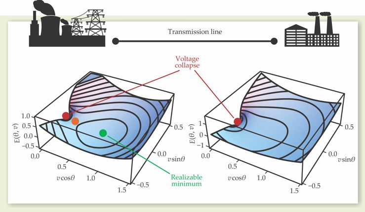
As the latter case illustrates, if the same system is too heavily loaded, voltage collapse is inevitable; a local minimum doesn’t even exist. ⁶ Although the energy functions in both cases describe an extremely simple two-node system, the same kind of evolution on an energy landscape applies equally well to realistic 40 000-node grids.

Synchronization of node frequencies

When the grid is in steady state, the local frequency deviations need not be zero but should be synchronized and relatively small at all nodes. Were that not the case, the phase differences θ_a − θ_b between connected nodes a and b would grow over time and the power flow between them would oscillate. The rapid transfers of electrical energy would cause rapid fluctuations in the rotational kinetic energy of large generators, and the resulting huge mechanical stresses could easily damage those expensive machines.

To ensure the continual synchronization of the frequency, a local stable minimum in the energy function (discussed in the box) must exist. Unfortunately, the equation is complex and nonlinear, which makes finding a minimum and verifying its stability to perturbation difficult. Building on results ⁷ from the 1980s, recent work reconsidered the energy function approach for an approximation that fixes the normalized voltage at all nodes to unity. ⁸ Interestingly, one can show that if a quadratic approximation for E(θ, v = 1) has a steady state with ∣θ_a − θ_b∣ < 1, then the original energy function has a stable minimum.

That statement has been proven for the case of tree-like networks and has also been empirically tested on meshed transmission grids. Finding the phase differences in the quadratic approximation can be reduced to solving the linearized and static form of equation 1—a computationally efficient process.

Electromechanical waves

The second-order derivative of θ_a in equation (1) creates some interesting phase dynamics that are described by a linear approximation:

(2) (2)

But in the case of large grids having fairly uniform properties, one need not take a discrete sum over connected nearest-neighbor nodes a and b. Instead, one can model the grid as a continuous system. ⁹ For long-length perturbations that span many nodes, that sum is approximated by a Laplacian of the now-continuous phase. The result is an electromechanical wave equation for θ having a constant phase velocity. Typical velocities are about 500 km/s in a moderately loaded grid that generates 100 MW every 100 km; the velocity decreases, though, as the grid becomes more heavily loaded.

Simulations of equation (2) reveal the wave nature of the electrical grid, including coherent frequency and phase oscillations that span it. ¹⁰ Those oscillations are manifestations of electromechanical standing waves—typically with frequencies less than a hertz and wavelengths around 2000 km. When the transmission grid is hit with a sudden, localized disturbance—the loss of a large generator, say—an electromechanical traveling wave propagates away from the source of the disturbance. Surprisingly, the greatest impact of the disturbance may be felt at locations remote from the source, as the wave constructively interferes with its reflection at the edge of the grid.

Statistical distance to failure

The grid is deemed reliable, at least according to (N − 1) feasibility, if it can operate in a state that’s robust to perturbations that arise when any of the grid’s major components fail. However, as renewable-energy generators are increasingly integrated into the grid, their time-intermittent outputs are likely to cause the grid to break down in ways not currently captured by that deterministic criterion. For example, the frequency controls (represented by the term in equation (1)) on large generators respond to fluctuating power output by changing their own outputs, which can potentially overheat a transmission line beyond its thermal limit.

New probabilistic methods, ¹¹ developed in the power engineering community and complemented by recent techniques based on the analysis of rare events, can measure the risk created by those fluctuations. ^{12 , 13} To see how, consider figure 3, a schematic representation of a test grid to which several renewable-energy generator nodes have been added. Each of those new nodes represents an axis along which the state of the electrical grid may fluctuate. In the space of possible deviations in output (such as the green plane S), some fluctuations in power preserve the grid’s integrity while others cause it to fail by, say, exceeding transmission-line capacities. Those limited capacities split the plane into feasible and infeasible regions.

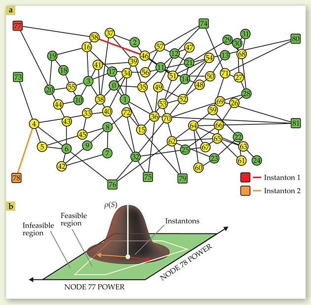
A probability distribution ρ(S) of deviations from the likely forecasted power (the white dot in figure 3) can be estimated. For a grid with a large number of renewable-energy nodes, evaluating the integral of the distribution over the infeasible region to obtain the probability of grid failure is a quite difficult problem. A computationally better strategy is to estimate the most probable fluctuation that resides in the infeasible region—the so-called instanton; borrowed from theoretical physics, ¹⁴ the term describes a special, most probable “instance.”

If the function ρ(S) is well behaved, finding the instanton is tantamount to maximizing the forecast error over the boundary of the globally feasible region. In general, that maximization is computationally hard. But if only thermal line limits are considered and physically reasonable approximations are used, the feasible region becomes a tractable polytope with 2N facets that correspond to the thermal limits for each direction of power flow of N transmission lines. Moreover, if the probability distribution is Gaussian, finding the instanton turns into a simple comparison of 2N analytical expressions, ¹² and existing (N − 1) methods for judging the grid’s reliability can be brought to bear. Generalizing the methods to account for other physical failures, such as a loss of synchronization or voltage collapse, is a significant research challenge.

Distribution grids and hysteresis

Because transmission-grid dynamics have been dominated by large centralized generators in the past, distribution-grid dynamics have traditionally been ignored. Grid operators can no longer afford to do that. New consumer devices—for instance, electric clothes dryers that disconnect to reduce real power consumption when the grid frequency falls below a preset threshold, and smart photovoltaic inverters that can quickly respond to local voltage deviations by injecting or consuming reactive power—will produce dynamics with the potential to significantly affect the transmission grid.

An awareness of distribution-grid dynamics is increasingly important because transmission grids are being operated closer to their stability limits. ¹⁴ But when the transmission grid is connected to tens of thousands of distribution circuits each serving tens of thousands of small electrical loads, device-level modeling becomes intractable. Fortunately, a limiting version of equation (1) yields a spatially continuous model that can be used to analyze many important examples of distribution-grid dynamics.

Take the case of induction motors, the small electrical motors that run air conditioning units or refrigerators. Figure 4a shows the state of a typical induction motor as a function of the voltage v at its terminals. For v ~ 1 (the voltage near its nominal distribution value), the motor is in a “normal” state, rotating at an angular frequency ω close to the grid frequency and consuming relatively low reactive power Q. If the voltage drops low enough, however, the motor enters a “stalled” state with ω falling to zero and Q rising high. The voltage of the normal and stalled states overlap, and the motor’s state is hysteretic. Transitions between those two states—and the dynamics of the motor in general—are primarily controlled by the motor’s rotational inertia.

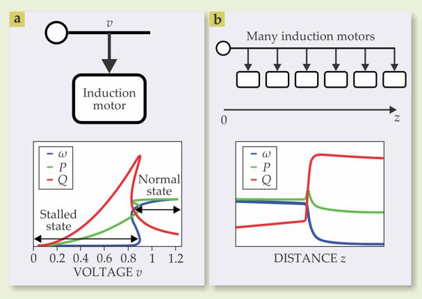
When a large number of such motors are spread along a distribution circuit, as illustrated in figure 4b, the large change in Q between an individual motor’s normal and stalled states induces long-range interactions between the states. The effect is most pronounced when a large disturbance in the local transmission system causes a drop in v large enough (to about 80% of its nominal voltage) and long enough (at least a few AC cycles) that all of the motors stall. When the transmission disturbance ends, the motors near the origin of the circuit, z = 0 in figure 4b, may quickly restart, but the collectively large Q from the more distant stalled motors holds down v for large z.

The result is the spatial segregation of normal and stalled states across a phase boundary. The circuit recovers to a fully normal condition when the phase boundary propagates to larger z—a situation reminiscent of the dynamics of a first-order phase transition. What’s more, simulations have shown that the phase boundary behaves like a soliton, maintaining a roughly constant shape as it propagates at nearly constant speed. ^{15 , 16}

A glimpse of the future

The electrical grid is currently undergoing revolutionary changes. Here, we outline a few technologies we believe will prove influential in the workings of tomorrow’s grid.

‣ Phasor measurement units are finally bringing synchronous detection of voltage and current to the grid. The GPS time-stamped, high-speed, near real-time data those devices provide will reveal grid dynamics with much higher spatiotemporal resolution than has previously been possible. (See http://www.eia.gov/todayinenergy/detail.cfm?id=5630 .)

‣ Flexible AC transmission (FACT) devices use fast-switching power electronics to provide nearly instantaneous control of reactive power injections, AC voltage levels, and, perhaps most importantly, control over real power flows through AC and DC transmission lines. Although so-called phase-shifting transformers can already electromechanically control the flow of real power over AC transmission lines, that control is relatively slow. Indeed, line-by-line control of real power flows is not possible in a FACTs-free transmission system. FACT devices will provide flexibility and control, but they’ll also present a challenge to grid operators, who need to understand the fast dynamics the devices will excite. (See http://spectrum.ieee.org/energy/the-smarter-grid/flexible-ac-transmission-the-facts-machine .)

‣ Large-scale electrical energy storage devices will potentially simplify grid operations by relaxing the need for instantaneous power delivery. Energy storage devices are expensive, though. What’s more, new algorithms are needed to optimally place and operate them to ensure the grid’s reliability. (See http://science.energy.gov/~/media/bes/pdf/reports/files/ees_rpt_print.pdf .)

In this article, we have emphasized the physicist’s view of the electrical grid. While that perspective provides an intuitive understanding of the grid’s behavior, its broader impact will be to enable the development of better methods for monitoring and controlling that behavior as the grid becomes smarter and more autonomous. Nonetheless, a physics analysis of the grid is, by itself, insufficient for laying the groundwork for tomorrow’s technologies. It should be coupled with complementary methods from operations research, computer science, control theory, machine learning, and electrical power engineering. We expect the most significant advances to come from combining those disciplines.

References

1. B. A. Carreras et al., Chaos 14, 643 (2004); https://doi.org/10.1063/1.1781391
R. Pfitzner, K. Turitsyn, M. Chertkov, 2011 IEEE Power and Energy Society General Meeting, IEEE, Piscataway, NJ (2011), p. 1.2. D. S. Callaway, I. A. Hiskens, Proc. IEEE 99, 184 (2011) and references therein. https://doi.org/10.1109/JPROC.2010.2081652
3. J. Lavaei, S. H. Low, IEEE Trans. Power Syst. 27, 92 (2012); https://doi.org/10.1109/TPWRS.2011.2160974
D. Bienstock, M. Chertkov, S. Harnett, arXiv:1209.5779 ; and references therein.4. P. Kundur, Power System Stability and Control, McGraw-Hill, New York (1994).
5. C. De Marco, A. Bergen, IEEE Trans. Power Syst. 34, 1546 (1987). https://doi.org/10.1109/TCS.1987.1086092
6. B. M. Weedy, B. R. Cox, Proc. IEE 115, 528 (1968);
V. A. Venikov et al., IEEE Trans. Power Appar. Syst. 94, 1034 (1975). https://doi.org/10.1109/T-PAS.1975.319377. A. R. Bergen, D. J. Hill, IEEE Trans. Power Appar. Syst. 100, 25 (1981). https://doi.org/10.1109/TPAS.1981.316883
8. F. Dörfler, M. Chertkov, F. Bullo, Proc. Natl. Acad. Sci. USA 110, 2005 (2013). https://doi.org/10.1073/pnas.1212134110
9. M. Parashar, J. S. Thorp, C. E. Seyler, IEEE Trans. Circuits Syst. I: Regular Pap. 51, 1848 (2004). https://doi.org/10.1109/TCSI.2004.834480
10. A. Chakrabortty, J. H. Chow, A. Salazar, IEEE Trans. Smart Grid 2, 68 (2011). https://doi.org/10.1109/TSG.2010.2093586
11. F. Alvarado, I. Dobson, Y. Hu, IEEE Trans. Power Syst. 9, 918 (1994). https://doi.org/10.1109/59.317655
12. M. Chertkov, F. Pan, M. Stepanov, IEEE Trans. Smart Grid 2, 162 (2011). https://doi.org/10.1109/TSG.2010.2090912
13. G. Falkovich et al., Phys. Rev. E 54, 4896 (1996). https://doi.org/10.1103/PhysRevE.54.4896
14. D. H. Popović, I. A. Hiskens, D. J. Hill, Int. J. Electr. Power Energy Syst. 20, 475 (1998). https://doi.org/10.1016/S0142-0615(98)00011-8
15. D. Wang, K. Turitsyn, M. Chertkov, arXiv:1209.5776 .
16. C. Duclut, S. Backhaus, M. Chertkov, arXiv:1212.0252 .
More about the authors
Scott Backhaus and Michael Chertkov are physicists at Los Alamos National Laboratory and the New Mexico Consortium.