From the archives: Analyzing atmospheric behavior
DOI: 10.1063/PT.3.2418
Editor’s note: Physics is an integral part of atmospheric science, whether one deals with forensic investigations (as in the article on page 32 ), local meteorology, climate change, or other planets’ atmospheres. Forty-four years ago, Hans Panofsky made the case that most meteorologists are really physicists in disguise.
Thirty five years or so ago, meteorologists practiced a descriptive science; they looked at weather maps and moved “highs” and “lows” around without understanding much of what they were doing. But now, meteorology having become a physical science, a discussion of the applications of physics to atmospheric problems includes most of meteorology. I shall not attempt here to present a complete catalog of the applications of physics to atmospheric studies. I shall limit myself to indicating the uses of hydrodynamics and thermodynamics, both needed in such basic problems as weather forecasting and explaining the general circulation. Some kinds of problems have been satisfactorily solved, and others need much additional work.
Variables and equations
If we ignore, for the moment, changes in atmospheric composition, the four basic variables are pressure p, temperature T, density ρ, and the three-dimensional wind velocity V. Four equations relate these variables:
p = RρT (1)
cp dT/dt − 1/ρdp/dt = C + I (2)
∇ · ρV + ∂ρ/∂t = 0 (3)
dV/dt = 2V × ω + g − 1/ρ∇p + Fr (4)
These equations were first written in 1904 by Wilhelm Bjerknes, 1 in much the same form as we now use them. Equation 1 is the question of state for dry air, in which R is the gas constant. In equation 2, a statement of the first law of thermodynamics, cp is heat capacity at constant pressure, C the rate of energy addition by “eddy” conduction, and I the rate of energy addition by radiation. Equation 3 is the equation of continuity, which states, for our purposes, that vertical shrinking is accompanied by increase in density; the first term is the horizontal divergence and the second term the vertical divergence. Equation 4 is Newton’s second law for a rotating body, in which ω is the rate-of-rotation vector of Earth, g is the force of gravity per unit mass, and Fr is “eddy” friction. We have here omitted molecular conduction and molecular friction, because these terms are usually small compared to the corresponding “eddy” terms.
Although constant-composition models of the atmosphere can solve some useful problems (for example, forecasting wind fields in the middle latitudes for 24–48 hours), the composition of the real atmosphere varies, affecting the equations. Many mathematical models of atmospheric systems contain additional variables, permitting composition to change. We denote all these variables by qi, the mass fraction of the ith constituent, and we write a conservation equation

for each qi. Si measures all sources and sinks of qi, and Di measures the gain or loss by eddy diffusion. We have neglected molecular diffusion.
Water vapor is the most important composition variable. (Assumption of a dry atmosphere makes prediction of rain very difficult!) If water vapor is taken into account, qi is the specific humidity, and equations 1 and 2 change. The effect on equation 1 is simply a minor correction to the ideal-gas law, but the effect on equation 2 can be profound: First, water vapor can condense, adding heat to the air; second, water vapor affects the radiative fluxes, in both the visible and the infrared regions, changing I significantly.
Even if water vapor is included as a variable, we have not properly predicted clouds. We still need to include other qi’s to describe the liquid water in the air, and perhaps even separate equations to describe the behavior of different-size drops. Clouds have, thus far, not been properly described in large-scale mathematical models of the atmosphere. In addition to water vapor, other qi’s may become important for special problems. If, for example, we are to model the stratosphere, the concentration of ozone must be permitted to vary and affect the radiation-energy term in equation 2.
We have all heard talk of how industry will inflict doom on civilization by changing the climate. 2 , 3 , 4 This doom will be caused either by putting too many particles into the atmosphere, which will reflect too much light and cause all the oceans and land to freeze from pole to pole, or by putting too much carbon dioxide into the atmosphere, thus warming it, melting the polar caps, and covering Earth with 300 feet of water.
Neither the concentration of particles nor of carbon dioxide is normally included in the meteorological equation. These variables clearly affect terms in the original equations. Treating particles is particularly difficult, because we don’t know much about their optical properties—do they reflect or absorb light?
Problems of scale
The atmosphere contains motions on all scales, from millimeters to thousands of kilometers. The same equations apply to problems on all these scales, from small convective clouds to the global circulation; we can neglect different terms for each case. For large systems, vertical velocities are relatively small, and vertical acceleration can always be neglected, compared to gravitational acceleration, in equation 4. Consistent with this approximation, the horizontal velocity divergence is often near zero. For very small-scale motions with time scales much less than a day, such as small eddies and clouds, Earth’s rotation can be neglected. Middle-size or “mesoscale” motions, such as lake storms, where no important simplifications are possible, are the most difficult motions to handle. And weather forecasts over a 3- to 12-hour period are the hardest to make, because mesoscale motions are involved; we can make simplifications for predictions over longer periods.
For any problem, we prescribe an initial field of motion, an initial temperature, and perhaps other variables on a particular scale; motions on all smaller scales are smoothed out. We take data from this smoothed field (usually at equally spaced grid points) and integrate the basic equations numerically.
We cannot, however, ignore the smaller-scale motions or eddies. Because the equations are nonlinear, these motions can interact with the main motion. Physically speaking, small-scale motion can affect larger-scale fields by mixing. Heat is carried from the warm to the cold air by the eddies. This is the reason for the C term in equation 2. The eddies also remove momentum from the atmosphere during mixing; this momentum transfer is included in the eddy-friction term of equation 4. And the mixing of air that is rich in qi with air that is poor in qiwill probably result in transport of qi; this transport is represented by D in equation
These eddy terms C, Fr, and D can be very tricky. They must either be specified a priori or related to other variables in the problem. The latter approach has been fairly successful close to the ground, but is quite difficult elsewhere, and eddy terms are sometimes omitted entirely above the lowest kilometer or so.
Solutions
Before we had large electronic computers we generally used perturbation methods to linearize the equations. First, a simple, steady mean field of wind, temperature, and humidity was assumed, and then small perturbations were superimposed. The perturbation properties were then investigated with the aid of the equations.
The results were wave equations, which determined the complex wave speed of the perturbations. If the wave velocities had positive imaginary parts, the wave would have exponential amplification factors and therefore be unstable. The amplification factors were functions of the perturbation wavelengths; for certain wavelengths, the factors were a maximum, and these waves were the most unstable.
Perturbation studies (which are still being done by some meteorologists 5 ) showed that two distinct types of instability exist. The first type, associated with horizontal distribution of wind and temperature, produces disturbances with horizontal dimensions of the order of thousands of kilometers but with vertical dimensions of only the order of kilometers. The second type, associated with vertical wind and temperature gradients, produces disturbances with horizontal and vertical dimensions of about one to three kilometers. Between these rather widely separated systems of motion the atmosphere is relatively stable. The kinetic energy of atmosphere circulations, then, is not uniformly distributed over different scales but rather is concentrated in horizontal dimensions of either thousands of kilometers or a few kilometers, with a gap between.
Mathematical models
The meteorological equations have been used, in their general, nonlinear form, to explain and forecast weather as well as to evaluate changes produced, either deliberately or inadvertently, by human activity. If we want to explain the characteristics of atmospheric motions (why, for example, there can be a snow squall in Buffalo when it is clear in Niagara Falls), then we use simplified data to establish the initial conditions.
The bottom boundary of the atmosphere can be treated in various ways; it can be simple and fixed, or, for long-period studies, it may change. If the boundary is a land surface, we can assume it will remain stationary throughout the integration period. If the boundary is the ocean, the atmosphere may cause a change in its temperature, which subsequently affects the atmosphere in another place. In the last few years, models have been developed that treat atmosphere and ocean as a single system (see
If we want to forecast the properties of atmospheric systems, integration of the equations must start from real observations. Adequate observations are at present usually available only over limited regions, and rather artificial boundary conditions must therefore be imposed. The effect of these conditions gradually spreads into the volume that we are interested in, and produces errors in the forecast; even an infinitesimal error in the original data causes instabilities in the system, so that after about two weeks we have only error.
To evaluate manmade changes in weather and climate, we can use either the first (simplified-data) or second (real-data) method. Initial conditions are altered to reflect the changes in atmosphere caused by pollution or by intentional addition of contaminants. Using the first method, we can study long-period effects; so far, the integration has been carried out over more than a year. As we have noted, the second method becomes useless after about two weeks.
Progress report
How successful have we been in applying the meteorological equations? We have been most successful with large-scale and very localized phenomena, and we have somewhat less satisfactory results for mesoscale systems.
Global circulations have been explained rather well. We now “understand” the general circulation and general characteristics of temperature distributions, as well as the statistical characteristics of traveling cyclones, anticyclones (high-pressure areas), and upper-air waves that have wavelengths of the order of 103 kilometers and larger; we have made more progress here in the last 20 years than in any other area.
We also understand the general behavior of the water cycle, although clouds have been assumed rather than produced by the mathematical models. Some models, as we have noted, have even included ocean circulation, and some ocean characteristics, as yet unobserved because of the slowness of the circulation, have been inferred. But the effect on the climate and circulation of pollution-induced changes in composition has not yet been studied and is of the highest priority. Useful experiments require much more sophisticated treatment of clouds and radiation than has so far been possible.
All weather forecasting is now done by application of the equations to large-scale systems. We have been most successful for 24- to 48-hour forecasts in the middle latitudes; tropical forecasting is less satisfactory. Our greatest improvements have been for upper-air forecasting, which we can do quite accurately except for predicting rain. A problem in rain prediction is that we cannot yet consider water droplets of varying sizes in our models, and that observation of precipitation is usually on a smaller scale than the scale we use for our forecasts.
Meteorologists are now cooperating in a worldwide effort to extend the period of satisfactory large-scale forecasts to a week or longer by 1976; this is the Global Atmospheric Research Program (GARP). One part of this program will be the collection of truly global weather data, mainly with the aid of satellites. (In limiting our discussion here to hydrodynamics and thermodynamics, I have omitted recent developments in meteorological measurement, particularly from distant points. This branch of meteorology has made great progress in the last few years; with present theories of infrared radiation we can now estimate global temperature distribution, at all levels, from weather satellites.) In addition, intensive efforts to get at the difficult terms in the meteorological equations, both theoretically and through field experiments, will be made. Although we will still be limited to two weeks for accurate weather predictions, because of essentially irreducible minor errors in initial conditions, we hope to predict statistical properties of the weather further into the future.

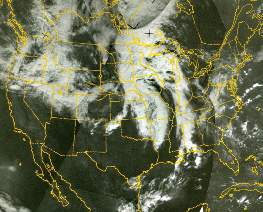
US cloud cover, 9 Oct. 1970. Montage of satellite photographs courtesy Vincent Oliver, National Environmental Satellite Center, National Oceanic and Atmospheric Administration.
On the mesoscale, we have used the equations to explain the development of hurricanes and their dependence on ocean temperature, and have made models that test the influence of cloud seeding on hurricane circulation. Our results here are controversial. Modifying individual clouds has been quite successful; we can predict accurately what the result of seeding a given cloud will be. But we don’t know what the real effect of such seeding is on a hurricane. This is a problem that we hope to solve in the next few years. Mesoscale predictions have usually been less satisfactory than large-scale predictions. A few types of circulation, such as lake-effect storms, sea breezes, and mountain waves, have been explained by the equations.
Air pollution can be treated as a mesoscale phenomenon. But here, the winds are assumed known, and only the conservation equation for the particular pollutant is used; the effect of the pollutant on the normal meteorological data is not considered. The eddy term Di produces substantial difficulties even here. In practice, we apply the conservation equation only when integrated over volumes, rather than at every point. The statistical distribution of the pollutant is assumed and its parameters found statistically. Accuracy of the estimates is limited mostly by errors in specifying the wind, which must be known on the mesoscale, and local variations caused by obstacles limit the accuracy. Uncertainty in the meteorological effects is, nevertheless, usually not an important limitation in air-pollution control.
On the small scale, explanation and prediction of the behavior of convective clouds has been particularly successful even though moisture must be dealt with in a quite sophisticated manner. A unique aspect of cloud study has been confirmation of predicted cloud development after seeding. On an even smaller scale, mathematical models have explained the statistical properties of eddies in the near-surface layer of the atmosphere.
Box. Ocean–atmosphere model
Empirical studies suggest that the ocean affects the atmosphere and vice versa. Jerome Namias of the Extended Forecast Department, National Oceanic and Atmospheric Administration (NOAA), points out that the ocean, once thermally disturbed, retains its heat for a long time. Then, once a seasonal change or air-mass movement begins, the ocean can enhance or inhibit storm development. Namias tells, for example, of an area about five to ten degrees north of Hawaii that appears to be a very sensitive index to North American weather. A very warm pool existed there during the summer and fall of 1968. Extremely strong cyclones (low-pressure disturbances) occurred there the following winter, and developed an upper-level trough. That winter was one of many aberrations in North American weather, including record-breaking waves and mudslides in California and extreme cold and snow in the Pacific Northwest. Namias does not believe the warm pool and subsequent aberrations are unrelated.
Meteorologists have for years been using mathematical models of the atmosphere to calculate climate variables. Now Syukuro Manabe and Kirk Bryan of the NOAA Geophysical Fluid Dynamics Laboratory, Princeton, have developed the first quantitative ocean–atmosphere model. Their calculation 1 , 2 reproduces many realistic climate features, even from rather arbitrary initial conditions. Manabe stresses that their model needs a great deal of additional work before it is useful for predicting weather or establishing quantitatively the kind of relationships that Namias and others have observed empirically.
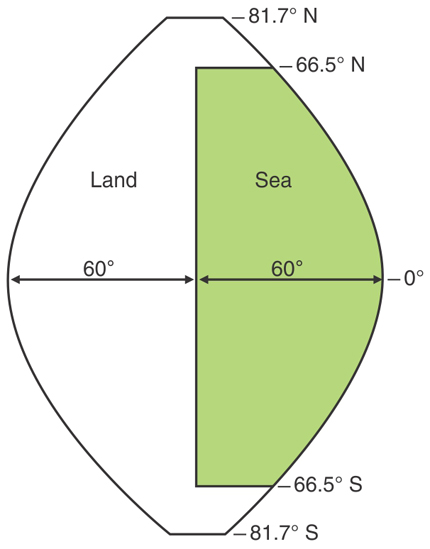
The atmospheric model that Manabe and Bryan use is similar to one developed by Manabe, Joseph Smagorinsky, and Robert Strickler; velocity, temperature, water vapor, and surface pressure are calculated at equally spaced (500 kilometers apart) grid points and at nine vertical levels. The ocean model is similar to that of Bryan and M. Cox; the calculations are done at five vertical levels and with grid spacing like that of the atmospheric model. This combined ocean–continent distribution of the model is, of course, highly simplified rather than closely analogous to real distribution (see figure above).

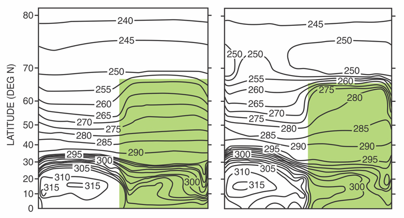
Surface-temperature patterns for the Manabe–Bryan model. Atmosphere-only stage is at left and final stage, including oceanic circulation, at right. Note isotherms over the northern part of the ocean; these isotherms have a northeast–southwest trend (as do real isotherms) in the right hand figure.

Ocean–continent configuration of the Manabe–Bryan model. East–west boundaries are meridians 120 deg apart, and the atmosphere at these boundaries is assumed cyclically symmetric. Northern and southern boundaries are insulated walls.
To make their results easier to interpret, Manabe and Bryan did their research in stages.
‣ The atmospheric model is studied without the effect of ocean circulation. At this stage, the ocean is simply an infinite moisture reservoir, with no heat capacity. Equilibrium is reached by numerically integrating the model from isothermal initial conditions.
‣ The ocean model is studied without feedback from the atmosphere. Surface-temperature, wind-stress, and precipitation distributions over the ocean are given by the first stage of the study and are assumed constant in time.
‣ The joint ocean–atmosphere model, in which the two systems interact fully, is studied. The average temperature of the upper 50 meters of ocean is used to set the lower-boundary temperature of the atmosphere. The rate of heat, momentum, and water supply that are computed for the atmospheric model serve as the upper-boundary condition for the ocean model.
An interesting result of the calculation is seen when the final state of the first stage is compared with the final state of the last stage. The comparison quantitatively demonstrates the effect of ocean currents in temperature distribution, humidity, and precipitation. The effect on surface-temperature distribution is seen in the figures
Referenes
1. S. Manabe, K. Bryan, J. Atmos. Sci. 26, 786 (1969).
2. S. Manabe, K. Bryan, Monthly Weather Review 97, 739, (1969).
References
1. W. Bjerknes, Meteorol. Z. 21, 1 (1904).
2. R. Bryson, “Is Man Changing the Climate of the Earth?” Saturday Review 50, 52 (1967).
3. R. Humphries, “The Imperiled Environment,” Vista 5, no. 5, 14 (1970).
4. F. Singer, Science 170, 125 (1970). https://doi.org/10.1126/science.170.3954.125
5. P. H. Stone, J. Atmos. Sci. 27, 721 (1970). https://doi.org/10.1175/1520-0469(1970)027<0721:ONGBSP>2.0.CO;2
More about the authors
Hans Panofsky is Evan Pugh Research Professor in the department of meteorology at Pennsylvania State University.


