Fractional Kinetics

Until about 10 years ago, expressions involving fractional derivatives and integrals were pretty much restricted to the realm of mathematics. But over the past decade, many physicists have discovered that a number of systems—particularly those exhibiting anomalously slow diffusion, or subdiffusion—are usefully described by fractional calculus. Those systems include charge transport in amorphous semiconductors, the spread of contaminants in underground water, relaxation in polymer systems, and tracer dynamics in polymer networks and in arrays of convection rolls.

Fractional diffusion equations generalize Fick’s second law and the Fokker–Planck equation by taking into account memory effects such as the stretching of polymers under external fields and the occupation of deep traps by charge carriers in amorphous semiconductors. Such generalized diffusion equations allow physicists to describe complex systems with anomalous behavior in much the same way as simpler systems.

Fractional calculus

Physicists are all familiar with the high-school calculus that introduces students to derivatives of integer order $n,{\text{d}}^{n}y/{\text{d}x}^n$ . Those derivatives and their inverse operations—integrations—provide the language for formulating and analyzing many laws of physics. But physicists generally aren’t taught about fractional-order derivatives, which might be formally expressed as, for example, ${\text{d}}^{1/2}y/\text{d}{x}^{1/2}$ . Is the fractional calculus all that difficult?

In fact, the calculus of fractional integrals and derivatives is almost as old as calculus itself. As early as 1695, Gottfried von Leibnitz, in a reply to Guillaume de l’Hôpital, wrote, “Thus it follows that ${\text{d}}^{1/2}x$ will be equal to $x\sqrt{\text{d}x:x},\dots$ from which one day useful consequences will be drawn.” About 300 years had to pass before what is now known as fractional calculus was slowly accepted as a practical instrument in physics. ¹ Before that acceptance, fractional calculus had to be more rigorously formulated. Important contributions to that end stem from the work of Pierre-Simon Laplace, Bernhard Riemann, Joseph Liouville, Oliver Heaviside, Arthur Erdélyi, and many others.

One way to formally introduce fractional derivatives proceeds from the repeated differentiation of an integral power: $$\frac{{\text{d}}^n}{\text{d}{x}^n}{x}^m=\frac{m!}{\left(m-n\right)!}{x}^{m-n}.$$ (1)

For an arbitrary power μ, repeated differentiation gives $$\frac{{\text{d}}^n}{\text{d}{x}^n}{x}^{\mu }=\frac{\Gamma \left(\mu +1\right)}{\Gamma \left(\mu -n+1\right)}{x}^{\mu -n},$$ (2) with gamma functions replacing the factorials. The gamma functions allow for a generalization to an arbitrary order of differentiation α, $$\frac{{\text{d}}^{\alpha }}{\text{d}{x}^{\alpha }}{x}^{\mu }=\frac{\Gamma \left(\mu +1\right)}{\Gamma \left(\mu -\alpha +1\right)}{x}^{\mu -\alpha }.$$ (3)

The extension defined by equation (3) corresponds to the Riemann–Liouville derivative. ² It is sufficient for handling functions that can be expanded in Taylor series.

A second, more elegant and general way to introduce fractional derivatives uses the fact that the nth derivative is an operation inverse to an n-fold repeated integration. Basic is the integral identity $${\displaystyle {\int }_a^x{\displaystyle {\int }_a^{y_1}\cdots }{\displaystyle {\int }_a^{y_{n-1}}f\left(y_n\right)\text{d}{y}_n\dots \text{d}{y}_1}}=\frac{1}{\left(n-1\right)!}{\displaystyle {\int }_a^x{\left(x-y\right)}^{n-1}f\left(y\right)\text{d}y}.$$ (4)

Clearly, the equality is satisfied at x = a, and it is not difficult to see iteratively that the derivatives of both sides of the equality are equal. A generalization of the expression allows one to define a fractional integral of arbitrary order α via $${ }_a{D}_x^{-\alpha }f\left(x\right)=\frac{1}{\Gamma \left(\alpha \right)}{\displaystyle {\int }_a^x{\left(x-y\right)}^{\alpha -1}}f\left(y\right)\text{d}y\left(x\ge a\right).$$ (5)

A fractional derivative of an arbitrary order is defined through fractional integration and successive ordinary differentiation. For additional elaboration, see box 1, which also discusses the relation between the value of the integration limit a and definitions for fractional differentiation based on the Laplace transform (when a = 0) and the Fourier transform (when a = −∞). The table above presents (for a = 0) several examples of semi-integrals and semi-derivatives, operations for which α = ± $\raisebox{1ex}{$1$}\!\left/ \!\raisebox{-1ex}{$2$}\right.$ .

Examples of fractional calculus with $\alpha =\pm \raisebox{1ex}{$1$}\!\left/ \!\raisebox{-1ex}{$2$}\right.$

In this article, we are generally concerned with fractional time derivatives, and we set a = 0, in effect choosing t = 0 as the beginning of the system’s time evolution. In particular, we note that the operator $${ }_0{D}_t^{1-\alpha }=\frac{\text{d}}{\text{d}t}{ }_0{D}_t^{-\alpha },$$ (6) with 0 < α < 1, plays a central role in generalized diffusion equations.

From Fick to fractional diffusion

The foundations of kinetics were established more than 150 years after the prophecy of Leibnitz, without the use of fractional calculus. In 1855, the young Adolf Fick, a pathologist at the University of Zürich, wrote a work entitled “Über Diffusion” (“On Diffusion”). The work was published in Poggendorf’s Annalen der Physik, the Physical Review Letters of that time. Fick started by observing that “diffusion in water confined by membranes is not only one of the basic factors of organic life, but it is also an extremely interesting physical process and, as such, should attract much more attention from physicists than it has so far.” Diffusion processes such as those considered by Fick, and processes that are described by fractional calculus, continue to fascinate physicists and others.

Fick was an experimental physiologist, but his work on diffusion was theoretical, and his approach would today be called a phenomenological linear-response theory applied to diffusion. In brief, the result of diffusion is known to be the equilibration of concentrations. Thus, particle current has to flow against the concentration gradient. In analogy with Ohm’s law for electric current, or with Fourier’s law for heat flow, Fick assumed that the current j is proportional to the concentration gradient, so that $$\mathbf{j}\left(\mathbf{r},t\right)=-\kappa \nabla c\left(\mathbf{r},t\right),$$ (7) an equation now known as Fick’s first law. Here, κ is the diffusion coefficient with dimension of L ²/T and c is the concentration. If, in addition, particles are neither created nor destroyed, then, according to the continuity equation, $$\frac{\partial c\left(\mathbf{r},t\right)}{\partial t}=-\nabla \cdot \mathbf{j}\left(\mathbf{r},t\right),$$ (8)

Combining Fick’s first law with the continuity equation gives Fick’s second law, also known as the diffusion equation: $$\frac{\partial c\left(\mathbf{r},t\right)}{\partial t}=\kappa {\nabla }^{2}c\left(\mathbf{r},t\right),$$ (9) which is a closed equation for the temporal evolution of the concentration.

Fick’s phenomenology missed the probabilistic point of view central to statistical mechanics. It was Albert Einstein who, 50 years after “On Diffusion,” first derived the diffusion equation from the postulates of molecular theory, in which particles move independently under the influence of thermal agitation. In his picture, the concentration of particles c(r, t) at some point r is proportional to the probability P(r, t) of finding a particle there. Thus, the diffusion equation holds when probabilities are substituted for concentrations.

If, for example, a particle is initially placed at the origin of coordinates in d-dimensional space, then its evolution, according to equation (9), is given by $$P\left(\mathbf{r},t\right)=\frac{1}{{\left(4\pi \kappa t\right)}^{d/2}}exp\hspace{0.17em}\left(-\frac{r^2}{4\kappa t}\right).$$ (10)

The mean squared displacement of the particle is thus $$〈r^2\left(t\right)〉={\displaystyle \int r^{2}P\left(\mathbf{r},t\right)}{\text{d}}^{3}r=2d\kappa t.$$ (11)

Note that the scaling form 〈r ²〉 ∝ t follows directly from the structure of the diffusion equation. That equation is second order in the spatial coordinates and first order in time: Changing the spatial scale by a factor of 3 corresponds to changing the time scale by a factor of 9.

In a variety of physical systems, however, the simple scaling pertinent to Fickian diffusion is violated. ^3,4 The mean squared displacement grows as $〈r^2〉\propto t^{\alpha }$ with the exponent α ≠ 1. A consistent generalization of the diffusion equation could still be second order in the spatial coordinate and have a fractional-order temporal derivative—for example, $$\frac{{\partial }^{\alpha }}{\partial t^{\alpha }}P\left(\mathbf{r},t\right)={\kappa }_{\alpha }{\nabla }^{2}P\left(\mathbf{r},t\right),$$ (12) where the dimension of the fractional diffusion coefficient κ _α is [L ²/T ^α ]. Equation (12) looks rather unusual. Does it make any sense? It does, as we now proceed to show.

Continuous-time random walks

Random walks and diffusion serve as an interface between kinetics on one hand and derivatives and integrals of fractional order on the other. The simplest model leading to normal diffusion is the random walk. Related models were introduced in Lord Rayleigh’s studies of isoperiodic vibrations (1880) and in Louis Bachelier’s analysis of stock-market fluctuations (1900). If a random walker strolling in one dimension moves a step of length a in either direction precisely when each unit time elapses, then the displacement after a large number of steps (that is, after a long time) will be distributed according to the Gaussian, equation (10).

In continuous-time random walks (CTRWs)—introduced in physics by Elliot Montroll and George Weiss—the condition that the steps occur at fixed times is relaxed. ⁵ Rather, the time intervals between consecutive steps are governed by a waiting-time distribution Ψ(t). In describing transport, the Ψ(t) distributions may stem from possible obstacles and traps that delay the particle’s jumps and thus introduce memory effects into the motion. If the mean waiting time between consecutive steps is finite, τ = ∫ t Ψ(t)dt < ∞, the CTRW is described by Fick’s diffusion equation, with the diffusion coefficient κ equal to α ²/2τ.

The situation changes drastically if the mean waiting time diverges, as is the case for power-law waiting-time distributions of the form $$\psi \left(t\right)\propto 1/{\left(1+t/\tau \right)}^{1+\alpha },$$ (13) with 0 < α < 1. ⁶ (See the article by Harvey Scher, Michael F. Shlesinger, and John T. Bendler, Physics Today, January 1991, page 26 .) Figure 1 compares the displacements of walkers undergoing simple random walks with those following CTRWs. The behavior for a CTRW is subdiffusive. The mean square displacement grows as $$〈x^2\left(t\right)〉\propto t^{\alpha }.$$ (14)

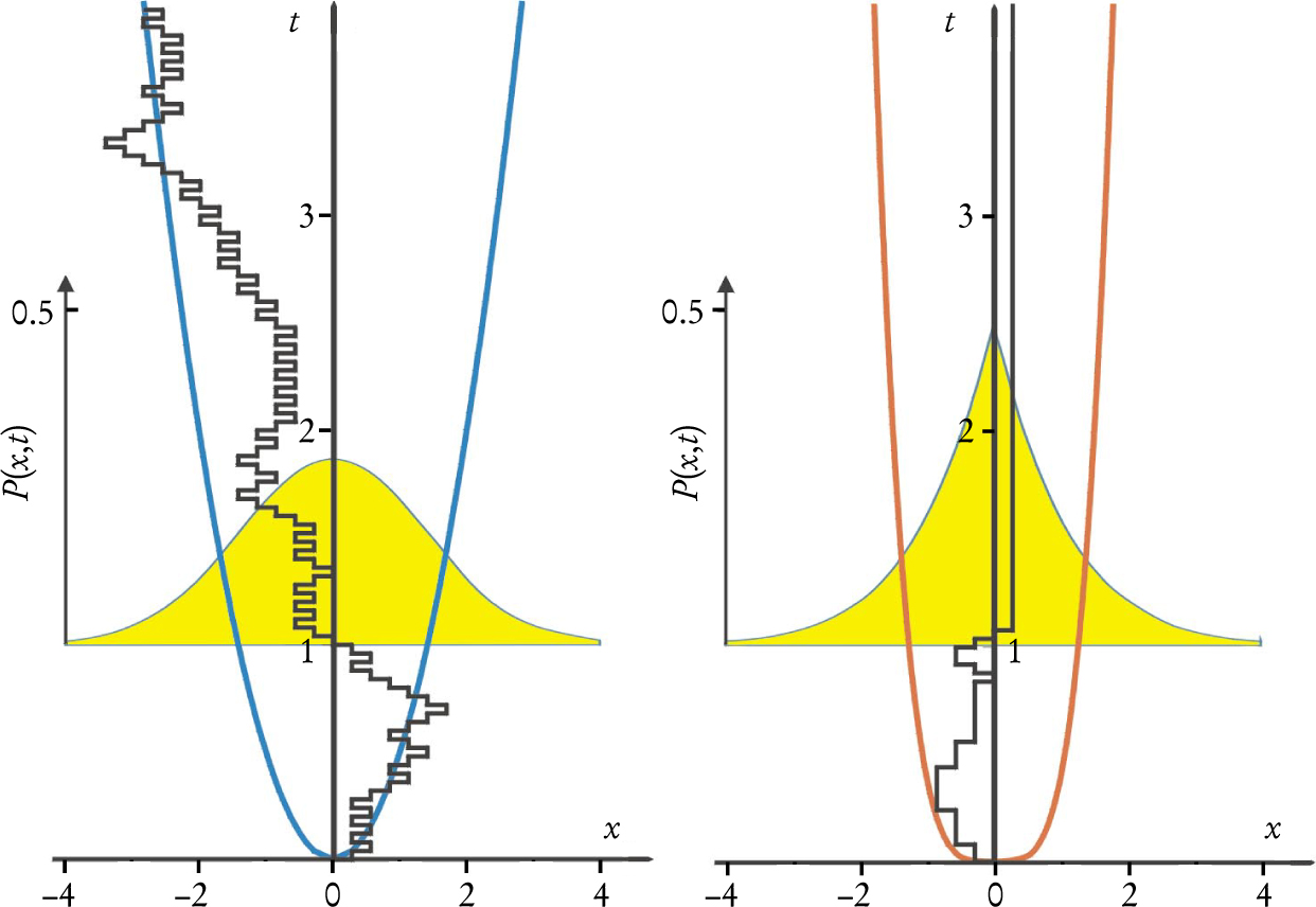
Transport phenomena in systems exhibiting subdiffusion have α < 1, whereas systems that exhibit superdiffusion have α > 1.

Fractional modifications of the commonly used diffusion and Fokker–Planck equations generate the scaling behavior seen in subdiffusive systems. Consider, for example, the fractional equation first introduced by Venkataraman Balakrishnan and by W. R. Schneider and W. Wyss: ⁶ $$\frac{\partial }{\partial t}P\left(x,t\right)={ }_0{\text{D}}_t^{1-\alpha }{\kappa }_{\alpha }{\nabla }^{2}P\left(x,t\right).$$ (15)

Equation (15) can be derived from the CTRW scheme along the lines used in Einstein’s work on Brownian motion, ⁷ and thus applies to all situations discussed adequately by CTRW. It treats systems that behave anomalously in a framework very much like the framework used for systems with normal diffusion, so that known solutions of the simple case can be easily generalized to the anomalous case. ⁸

Fractional Fokker–Planck equation

The standard diffusion equation accounts for a particle’s motion due to uncorrelated molecular impacts. In many cases, an external deterministic force is imposed on a system in addition to such random impacts. The Fokker–Planck equation considers both contributions. ⁹ It can be derived by combining Fick’s first law—expressed in terms of probability current and taking into account the external force—with the continuity equation. The probability current is $$\mathbf{j}\left(\mathbf{r},t\right)=-\kappa \nabla P\left(\mathbf{r},t\right)+\mu \mathbf{f}\left(\mathbf{r},t\right)P\left(\mathbf{r},t\right),$$ (16) where f is the external force acting on the particle and μ is the particle’s mobility. When the continuity equation is applied to the probability current, the Fokker–Planck equation follows: $$\frac{\partial P\left(\mathbf{r},t\right)}{\partial t}=\nabla \cdot \left(-\mu \mathbf{f}P\left(\mathbf{r},t\right)+\kappa \nabla P\left(\mathbf{r},t\right)\right).$$ (17)

In the absence of an external force, f = 0, the Fokker–Planck equation reduces to the standard diffusion equation.

In parallel to the diffusion case, one can generalize the Fokker–Planck equation to $$\frac{\partial P\left(\mathbf{r},t\right)}{\partial t}={ }_0{D}_t^{1-\alpha }\nabla \left(-{\mu }_{\alpha }\mathbf{f}P\left(\mathbf{r},t\right)+{\kappa }_{\alpha }\nabla P\left(\mathbf{r},t\right)\right),$$ (18) where μ _α is the fractional mobility.

In equilibrium, the current j must vanish. After expressing the force in terms of a potential function U(r), one may write the equilibrium probability distribution that satisfies equation (18) in the form $P\left(\mathbf{r}\right)\propto \exp \left(-{\mu }_{\alpha }U\left(\mathbf{r}\right)/{\kappa }_{\alpha }\right)$ . Now, for independent particles, the equilibrium probability is a Boltzmann distribution, so ${\kappa }_{\alpha }/{\mu }_{\alpha }=k_{B}T$ , a generalization of Einstein’s relation $\kappa /\mu =k_{B}T$ .

For example, consider a constant external force acting in the x direction. The force leads to a mean drift, ${〈x\left(t\right)〉}_f={\mu }_{\alpha }f{t}^{\alpha }/\Gamma \left(1+\alpha \right)$ , which is related to the force-free mean square displacement ${〈x^2\left(t\right)〉}_{f=0}=2{\kappa }_{\alpha }{t}_{\alpha }/\Gamma \left(1+\alpha \right)$ through $${〈x\left(t\right)〉}_f=\frac{1}{2}f\frac{{〈x^2\left(t\right)〉}_{f=0}}{k_{B}T}.$$ (19)

The expression above is the fluctuation-dissipation theorem, which holds for subdiffusion in the fractional Fokker–Planck framework.

Ornstein–Uhlenbeck processes in one dimension provide a second example. Such processes involve diffusion in the harmonic potential $U\left(x\right)=b{x}^2/2$ so that the force is f = −bx. The corresponding fractional Fokker–Planck equation is $$\frac{\partial P\left(x,t\right)}{\partial t}={ }_0{D}_t^{1-\alpha }\left({\mu }_{\alpha }b\frac{\partial }{\partial x}\left[xP\left(x,t\right)\right]+{\kappa }_{\alpha }\frac{{\partial }^2}{\partial x^2}P\left(x,t\right)\right).$$ (20)

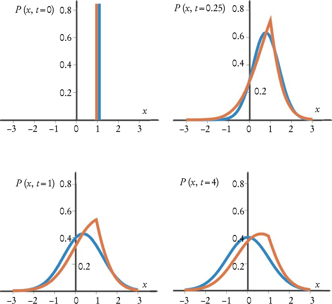
Figure 2 shows snapshots of the time-dependent probability distribution for particles originally at a well-defined location, according to both the fractional and conventional Fokker–Planck equations with harmonic potentials. In both cases, the asymptotic forms of the distribution are Gaussian, because the Fokker–Planck equations describe the relaxation of thermodynamic systems to equilibrium. In the fractional case, though, the distribution at finite times has a cusp characteristic of broad CTRW distributions.

In thermodynamic applications, one is mostly interested in mean values—for example, the mean particle position $<x\left(t\right)>={\displaystyle \int x}P\left(x,t\right)\text{d}x$ . In the regular case of simple diffusion in the harmonic potential U(x), there is a characteristic time τ given by τ ⁻¹ = b _μ . The evolution of the mean position satisfies $$\frac{\text{d}〈x\left(t\right)〉}{\text{d}t}=-{\tau }^{-1}〈x\left(t\right)〉.$$ (21)

It follows that 〈x(t)〉 decays exponentially toward equilibrium: 〈x(t)〉 = 〈x(0)〉 exp(–t/τ).

In the case of diffusion governed by the fractional Fokker–Planck equation, the mean displacement obeys $$\frac{\text{d}〈x\left(t\right)〉}{\text{d}t}=-{\tau }^{-\alpha }{ }_0{D}_t^{1-\alpha }〈x\left(t\right)〉,$$ (22) with ${\tau }^{-\alpha }=b{\mu }_{\alpha }$ , as is readily verified by multiplication of equation (20) by x and integration, followed by an integration by parts of the right-hand side. The solution of equation (22) can be expressed in terms of the Mittag–Leffler function E _α via $<x\left(t\right)>=<x\left(0\right)>E_{\alpha }\left(-{\left(t/\tau \right)}^{\alpha }\right)$ . The Mittag–Leffler function, illustrated in figure 3 for α = $\raisebox{1ex}{$1$}\!\left/ \!\raisebox{-1ex}{$2$}\right.$ , is a natural generalization of the exponential function; in particular, $E_1\left(-t/\tau \right)=\exp \left(-t/\tau \right)$ . Figure 4 compares the exponential relaxation of the mean position obtained in the case of normal diffusion with the slower relaxation described by the Mittag–Leffler function.

Applications

The regular Ornstein–Uhlenbeck process is a good model for the behavior of a diffusing particle trapped in optical tweezers: The tweezers create an approximately harmonic well. The corresponding relaxation patterns display exponential decays, as shown by Roy Bar-Ziv and colleagues from the Weizmann Institute of Science in Rehovot, Israel. Particles moving according to the fractional Ornstein–Uhlenbeck equation (equation (20)) should exhibit Mittag–Leffler relaxation. Rony Granek, from Ben-Gurion University, suggested that such relaxation would be observed for beads attached to a vesicle and held by optical tweezers. Walter Glöckle and Theo Nonnenmacher of the University of Ulm, Germany, used Mittag–Leffler relaxation in their analyses of rheology in polymeric systems and of rebinding experiments in proteins. This past year, a group led by Harvard University’s Sunny Xie used the fractional Ornstein–Uhlenbeck equation to describe the dynamics of protein molecules probed by electron transfer.

One can expect applications of the fractional Fokker–Planck equation in chemical and biological systems. As early as 1916, Marian Smoluchowski showed how the rates of chemical reactions can be determined by imposing boundary conditions on diffusion equations. Because the fractional Fokker–Planck equation handles boundary value problems in the same way as its regular counterpart does, it is a valuable tool for describing reactions in complex systems, as recently reported by groups led by Katja Lindenberg at the University of California, San Diego, and Bob Silbey at the Massachusetts Institute of Technology. ¹⁰

Many environmental studies are complicated by a poor understanding of the diffusion of contaminants in complex geological formations. Experiments point to anomalous diffusion. They suggest the need for fractional diffusion–advection equations, ¹¹ which may help scientists to understand and predict the long-term impact of pollution on ecosystems. ¹²

Detailed studies of the fractional Kramers problem represent another possible arena for the application of fractional kinetics. The problem concerns the escape of a particle over a potential barrier. First steps toward its solution have been achieved by Ralf Metzler and Yossi Klafter, both working at Tel Aviv University.

Fractional calculus can be applied to many areas of physics, other than fractional kinetics. In fact, fractional calculus was introduced in a heuristic manner long ago in rheology (for example, by Andrew Gemant in 1936) in an effort to describe linear viscoelasticity through the extension of the material-dependent constitutive equations used in the field. ¹³ Box 2 discusses examples of hierarchical structures whose dynamics are conveniently described with fractional derivatives. Many other examples of applications of fractional calculus to modern physics are presented in reference .

What about superdiffusion? Fractional generalizations of the diffusion and Fokker–Planck equations have been introduced for superdiffusion as well. Those equations, which apply spatial fractional derivatives rather than temporal ones, are intimately related to Lévy processes in space. George Zaslavsky has advocated using such equations to describe chaotic diffusion in Hamiltonian systems, and other applications have been discussed by Hans Fogedby and by Bruce West and Paolo Grigolini. ^1,14 We hasten to note, however, that superdiffusion is far from being completely understood.

The classical diffusion laws derived by Fick dominated physicists’ views on diffusion and transport for more than a century. But recent observations have clearly demonstrated that Fick’s laws have exceptions. Those exceptions, which have been termed strange kinetics, ³ require a completely fresh view of kinetic processes, based on random-walk approaches and on unconventional distribution functions (see the article by Joseph Klafter, Michael F. Shlesinger, and Gert Zumofen, Physics Today, February 1996, page 33 ). Fractional calculus helps formulate the problems of strange kinetics in a simple and elegant way.

References

1. R. Hilfer, ed., Applications of Fractional Calculus in Physics, World Scientific, River Edge, N. J. (2000).
2. K. B. Oldham, J. Spanier, The Fractional Calculus, Academic Press, San Diego, Calif. (1974);
K. S. Miller, B. Ross, An Introduction to the Fractional Calculus and Fractional Differential Equations, Wiley, New York (1993).3. M. F. Shlesinger, G. M. Zaslavsky, J. Klafter, Nature 363, 31 (1993).https://doi.org/10.1038/363031a0
4. J.-P. Bouchaud, A. Georges, Phys. Rep. 195, 127 (1990).https://doi.org/10.1016/0370-1573(90)90099-N
5. E. W. Montroll, G. H. Weiss, J. Math. Phys. 10, 753 (1969);https://doi.org/10.1063/1.1664902
E. W. Montroll, M. F. Shlesinger, in Nonequilibrium Phenomena II: From Stochastics to Hydrodynamics, J. L. Lebowitz, E. W. Montroll, eds., North Holland, New York (1984);
E. W. Montroll, B. J. West, in Fluctuation Phenomena, E. W. Montroll, J. L. Lebowitz, eds., North Holland, New York (1987).6. V. Balakrishnan, Physica A 132, 569 (1985);https://doi.org/10.1016/0378-4371(85)90028-7
W. R. Schneider, W. Wyss, J. Math. Phys. 30, 134 (1989).https://doi.org/10.1063/1.5285787. R. Metzler, J. Klafter, Phys. Rep. 339, 1 (2000).https://doi.org/10.1016/S0370-1573(00)00070-3
8. E. Barkai, Phys. Rev. E 63, 046118 (2001);https://doi.org/10.1103/PhysRevE.63.046118
I. M. Sokolov, Phys. Rev. E 63, 056111 (2001).https://doi.org/10.1103/PhysRevE.63.0561119. H. Risken, The Fokker–Planck Equation: Methods of Solution and Applications, Springer-Verlag, New York (1996).
10. S. B. Yuste, K. Lindenberg, Phys. Rev. Lett. 87, 118301 (2001);https://doi.org/10.1103/PhysRevLett.87.118301
J. Sung, E. Barkai, R. J. Silbey, S. Lee, J. Chem. Phys. 116, 2338 (2002).https://doi.org/10.1063/1.144829411. J. W. Kirchner, X. Feng, C. Neal, Nature 403, 524 (2000).https://doi.org/10.1038/35000537
12. R. Metzler, J. Klafter, I. M. Sokolov, Phys. Rev. E 58, 1621 (1998).https://doi.org/10.1103/PhysRevE.58.1621
13. C. Friedrich, H. Schiessel, A. Blumen, in Advances in the Flow and Rheology of Non-Newtonian Fluids, D. A. Siginer, D. De Kee, R. P. Chhabra, eds., Elsevier, New York (1999), p. 429.https://doi.org/10.1016/S0169-3107(99)80038-0
14. G. M. Zaslavsky, Chaos 4, 25 (1994);https://doi.org/10.1063/1.166054
H. C. Fogedby, Phys. Rev. Lett. 73, 2517 (1994).https://doi.org/10.1103/PhysRevLett.73.2517
More about the authors
Igor Sokolov is a professor of physics at Humboldt University in Berlin, Germany
Igor M. Sokolov, 1 Humboldt University, Berlin, Germany .
Joseph Klafter, 2 Tel Aviv University, Israel .
Alexander Blumen, 3 University of Freiburg, Germany .