Enrico Fermi and Quantum Electrodynamics, 1929–32
DOI: 10.1063/1.1496373
In 1926, shortly after the publication of Erwin Schrödinger’s wave mechanics papers, Enrico Fermi wrote a short article entitled “Arguments Pro and Con the Hypothesis of Light Quanta.” 1 Having carefully studied and mastered Schrödinger’s papers, Fermi declared in his paper that “at the present time the state of science is such that one can say that we lack a theory that gives a satisfactory account of optical phenomena.” He also listed the experiments that were convincingly explained by light’s particlelike character, such as the photoelectric and Compton effects, and those experiments that were readily understood in terms of wave theory, namely, interference and diffraction. The challenge, Fermi stated, was to elucidate the processes involved in the interaction of light with matter at the atomic level and to give intuitive explanations of macroscopic optical phenomena at the microscopic level.
Fermi met his own challenge in a series of papers that appeared in Rendiconti della academia national dei Lincei (1929–30), Annales de l’Institut Henri Poincaré (1931), Nuovo Cimento (1931), and Reviews of Modern Physics (1932). 1 In those papers, he formulated a relativistically invariant description of the interaction between charged particles and the electromagnetic field that treated both particles and the EM field quantum mechanically. Briefly: He first devised a simple, readily interpretable, Hamiltonian description of charged particles interacting with the EM field. Then, he showed how to quantize this formulation and how to exploit perturbation theory to describe quantum electrodynamic phenomena. Other physicists tackled the same problems, but none of the alternative formulations—Werner Heisenberg and Wolfgang Pauli’s, in particular—combined the simplicity, transparency, and thoroughness of Fermi’s approach.
Walter Heitler was among the physicists influenced by Fermi’s formulation of quantum electrodynamics (QED). Heitler’s book Quantum Theory of Radiation , which first appeared in 1936, taught physicists during the late 1930s and 1940s how to calculate cross sections for electrodynamic processes. In the book, after paying lip service to Paul Dirac’s classic 1927 papers, Heitler based his approach to the quantization of the EM field on Fermi’s articles.
Fermi’s formulation was also Richard Feynman’s point of departure in his 1939 PhD dissertation at Princeton University. Using Fermi’s formulation of quantum electrodynamics, Feynman gave a description of the motion of charged particles when the effects of the radiation field are integrated out.
Another physicist who exploited Fermi’s formulation of QED was Victor Weisskopf. Weisskopf realized that the Lamb shift could be interpreted as the effect of the zero point energy vacuum fluctuations of the EM field on the motion of the electron in the hydrogen atom.
Fermi showed how to handle the gauge conditions when the electromagnetic field is described by vector and scalar potentials. His treatment was the first to explain how to fix gauges in quantized gauge theories. He also indicated under what circumstances the intuitive picture of a photon as a mass less, spin-1 particle-like entity that moves with velocity c was appropriate. And in a 1932 paper with Hans Bethe, Fermi helped establish the perturbation theoretic picture that depicts the electromagnetic interaction between charged particles as stemming from the exchange of photons. (For more about Bet he’s collaboration with Fermi, see the article by bethe on page 28.)
Rendiconti lincei
In his preface to the QED articles in the first volume of Fermi’s collected papers, Edoardo Amaldi recounted that Fermi started studying the quantum theory of radiation during the winter of 1928–29. 1 First, Fermi mastered Dirac’s two 1927 papers that had laid the foundations of the subject. Then, he familiarized himself with the papers of Pascal Jordan and Oskar Klein (1927) and of Jordan and Eugene Wigner (1928). In those papers, Jordan, Klein, and Wigner recovered the wave-mechanical description of a system of N identical nonrelativistic bosons and fermions in 3N-dimensional configuration space by “quantizing” an appropriate Schrödinger equation that they took to describe a wave field. Fermi also read—and was impressed by—Jordan and Pauli’s 1928 paper in which they formulated a quantization procedure for the free EM field in a relativistically invariant manner.
In the first of his 1927 papers, Dirac dealt with the problem of how an atom interacts with the EM field. Photons, according to Dirac, were particles of zero rest mass that obey Bose–Einstein statistics. To describe the interaction between charged particles and photons, he introduced a Hamiltonian that conserved the number of photons. But such a Hamiltonian could describe neither the spontaneous emission of photons nor their absorption. Dirac circumvented this limitation by assuming that zero-energy photons were special (on the grounds that they are unobservable), and he characterized the vacuum as a state with an infinite number of photons of zero energy and zero momentum. Furthermore, he stipulated that in any physical state, an infinite number of such photons exist.
Dirac went on to consider photon emission as a transition from the vacuum state to a state with an additional single photon of finite momentum and energy. Photon absorption consisted of the reversed transition. By imposing a limiting procedure in which the number of zero-energy photons became infinite and the matrix element for a transition from the vacuum state to a state with a photon of finite energy became vanishingly small, Dirac could account for the emission and absorption of photons, including spontaneous emission.
In the last, brief section of his paper, Dirac turned to the interaction of an atom with the EM field from the wave’s point of view. He adopted the Coulomb gauge, in which the EM field is described by a transverse vector potential (with zero divergence) that he considered to be a noncommuting variable. He could then show that the particle and wave approaches were equivalent provided the interaction in the wave formulation is taken to be
Amaldi recalled that “the method used by Dirac did not appeal to Fermi, who preferred, as he did very often, to recast the theory in a form mathematically more familiar to him.” 1 But it was probably not so much the mathematical aspects of dirac’s formulation that failed to appeal to Fermi, but the physical approach. Although in Dirac’s paper the notion of a photon was evident, its connection to the quantization of the em field was unclear, because dirac’s formulation did not rest on a well-defined quantization procedure for the EM field. Moreover, the formulation’s relativistic invariance was not obvious. Nor could the formulation deal with the problem of how the EM field reacts when a photon is emitted—a problem that Fermi had identified in 1926 after reading Schrödinger’s papers.

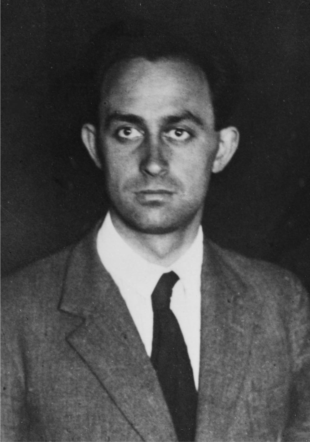
Enrico Fermi was a lecturer at the university of florence in 1926 when he wrote “arguments pro and con the hypothesis of light quanta,” his first published step toward understanding how radiation and atoms interact at the quantum level. The following year, he was elected a professor of theoretical physics at the university of rome, a post he held until 1938.
(Courtesy of aip emilio segrè visual archives.)
Despite Fermi’s misgivings about Dirac’s treatment, it is clear from the problems he subsequently addressed that fermi had noted and adopted dirac’s desiderata for any acceptable QED theory. Such a theory, Dirac proposed, should
correctly take into account that electromagnetic forces are propagated with the velocity of light instead of instantaneously
describe the production of an EM field by a moving electron
describe the reaction of the EM field to the electron
satisfy all the requirements of special relativity.
In his first article on QED, which appeared in Rendiconti Lincei in 1929, Fermi stated that he wanted to formulate the equations of motion of classical electrodynamics in such a way that they could readily be translated into a quantum form. His approach was to describe the EM field (assumed to be contained in a large cavity of volume Ω) in terms of a scalar potential v and a vector potential U that satisfy:
Expressed in terms of the Fourier coefficients Qs and qs , the equations of motion, equations
In effect, equations
Fermi concluded his first QED paper by writing down the Hamiltonian that yielded the equations of motion of both the EM field (equations
Pauli, after reading Fermi’s paper, wrote Jordan: “I have studied Fermi’s Rendiconti della Accademia dei Lincei (May 1929) electrodynamics article very carefully. It does not depend at all on Heisenberg and my article and is methodologically interesting although it doesn’t produce any new results.”
Another methodologically interesting and important point was expounded in Fermi’s second Rendiconti Lincei paper. There, Fermi indicated that when electrodynamics is quantized, the gauge condition

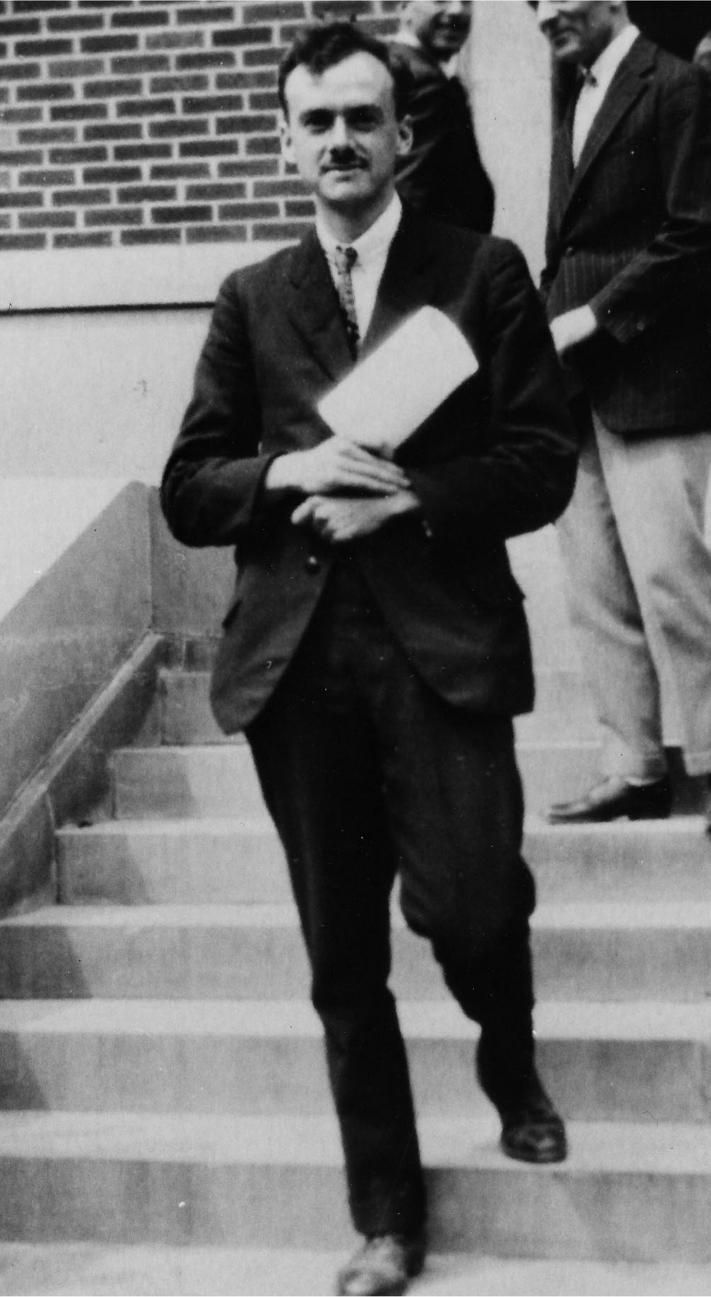
Paul Dirac wrote two papers in 1927 that laid the groundwork for Fermi’s subsequent investigations into quantum electrodynamics. Dirac became a fellow of St. John’s College, Cambridge in 1927, and, five years later, was elected to the same Cambridge University chair held previously by Isaac Newton.
(Courtesy of AIP Emilio Segrè Visual Archives.)
Early in 1929, Fermi heard about Weisskopf and Wigner’s work on the theory of linewidths, a problem of great interest to Fermi. Just after the advent of wave mechanics, Fermi had tried unsuccessfully to account for the lifetime of an atom’s excited state and for the natural linewidth of the emitted radiation. He clearly mastered Weisskopf and Wigner’s paper. In fact, the paper became the key that helped Fermi to explain interference and other undulatory light phenomena from a microscopic viewpoint.
As Fermi tackled these and other problems, he would share and explain his insights. According to Amaldi, Fermi
taught his results to several of his pupils and friends including Amaldi, Majorana, Racah, Rasetti and Segrè. Every day when work was over he gathered the various people … around his table and started to elaborate before them, first the basic formulation of quantum electrodynamics and then, one after the other, a long series of applications of the general principles to particular physical problems. A striking feature of Fermi’s method of working on a theoretical problem in public (so to speak) and of teaching at the same time, was the way in which he could say out loud what he was thinking, proceeding at a steady unhesitating pace; never going extremely fast, but never failing to make progress.
1
Annales de l’Institut Henri Poincaré
In April 1929, Fermi presented his findings in a course at the Henri Poincaré Institute in Paris. Summarized in the institute’s Annales, the lectures elaborated on the physical content of Fermi’s approach. He first considered the interaction of a single charged particle with the EM field. When the particle’s motion is prescribed (that is, when v = dX/dt is specified), it is possible to integrate the equations analogous to equation
However, the principal thrust of the Paris lectures was to establish QED as a readily usable theory. To do so, Fermi showed how perturbation theory could be recast to analyze and calculate transition amplitudes in an almost algorithmic manner. Until the spring of 1929, no one had given a fully quantum-mechanical formulation of electrodynamic processes. The computation of the cross sections for the photoelectric effect, Compton scattering, and so on all depended on either semiclassical or correspondence principle approaches. What Fermi did was to demonstrate how all these processes could be given a fully quantum-mechanical treatment and how perturbation theory should be handled to derive the cross sections for the processes.
Fermi’s point of departure was the Schrödinger-Dirac perturbation theory in which the wavefunction for the system, which satisfïes the Schrödinger equation
How to use these equations to compute the ak for various physical processes was the subject matter of the lectures that Fermi gave in 1930 at the University of Michigan Summer School in Ann Arbor. The content of these lectures constituted the bulk of his 1932 article in the Reviews of Modern Physics.
Reviews of modern physics
After introducing his formulation of QED in Rendiconti Lincei, Fermi turned to the formulation’s applications and implications. The first problem he addressed was that of the linewidth of the radiation emitted by an atom. Weisskopf and Wigner had derived an approximate solution, which Max Born evidently communicated to Fermi. The Weisskopf-Wigner solution played an important role in the examples that Fermi subsequently examined in his Michigan lectures.
Fermi’s model of spontaneous emission of radiation was as follows. At time t = 0, a two-level atom is in an excited state. No photons are present. After a certain time, the atom drops into its ground state and emits a photon. Fermi set himself the objective of computing the probability amplitude, a E(t), that the atom is still in its excited state at time t . Fermi showed that an approximate solution,
Fermi disliked complicated theories and avoided them as much as possible… . His article on the Quantum Theory of Radiation in the Reviews of Modern Physics (1932) is a model of many of his addresses and lectures: nobody not fully familiar with the intricacies of the theory could have written it, nobody could have better avoided those intricacies…
2
Fermi’s second example in the Reviews of Modern Physics article was the propagation of photons in the vacuum. The work of one of his students, Giulio Racah, had laid the problem’s groundwork. Fermi considered two two-level atoms: A, located at the origin, and B, located a distance r away. Initially, A is in an excited state whose lifetime 1/ΓA is assumed to be short enough that A emits a photon at a definite time and place. Fermi further assumed that B is in its ground state and that the mean life of the state to which B is excited by photon absorption is very long. Because 1/ΓA is very short, the line emitted by A is very broad; Fermi considered it as part of the continuum. B, however, absorbs a very sharp line. Fermi examined the probability amplitude, a GE , for finding the following at time t: atom A in the ground state, atom B in the excited state, and no photons present. When r is much larger than the wavelength of the emitted radiation, Fermi showed that
The next problem Fermi treated in his Reviews of Modern Physics article, the theory of Lippmann fringes, depended on the previous analysis. He used atom A as a localized source for the emitted photon, and atom B for the detector.

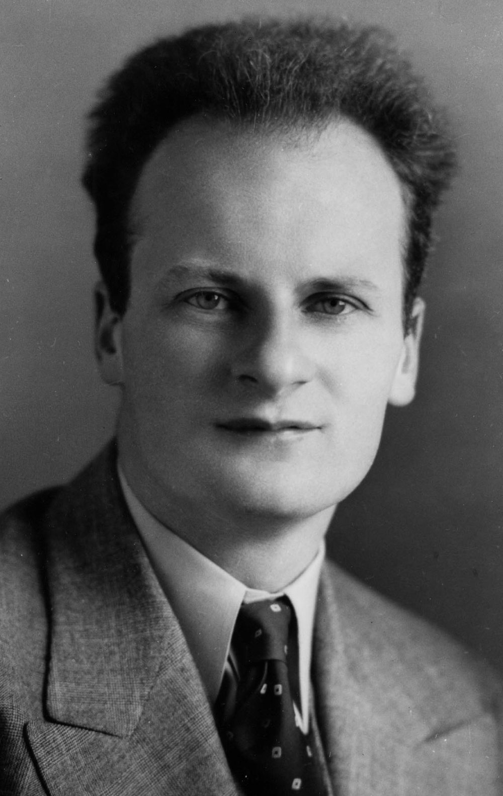
Hans Bethe visited Fermi in Rome in the spring of both 1931 and 1932. A result of their collaboration was a 1932 paper that treated the force between two charged particles as arising from the exchange of photons. Bethe was based at the University of Munich at the time.
(AIP Emilio Segrè Visual Archives, Physics Today Collection.)
Of the further examples, it is clear that Fermi thought that two were especially important: Thomson and Compton scattering. He wanted to illustrate how perturbation theory yielded the by then familiar cross sections for these processes, and to indicate how QED recovered the classical Thomson limit for the scattering of long wavelength radiation off free electrons. In particular, he pointed out that in the nonrelativistic approximation, it was the A 2 term that was responsible for the effect.
In both his Michigan Summer School lectures and in his Reviews of Modern Physics paper, Fermi discussed the Dirac equation extensively. At the time Fermi submitted the paper, Dirac had formulated his hypothesis that all the negative energy states were filled and that holes in the negative energy sea corresponded to protons. Fermi referred to Igor Tamm’s and Robert Oppenheimer’s work that pointed out the difficulty with that interpretation: The hydrogen atom would be unstable because protons and electrons could annihilate via two-photon emission. Fermi also stressed that the contributions of the negative energy states had to be included to derive the Klein-Nishina formula and to recover the Thomson limit from it.
In 1932, Fermi and Bethe set out to derive the interaction potential between two charged particles, including magnetic and retardation effects. The problem, which was controversial at the time, had been tackled by Christian Møller, Gregory Breit, and others. Historians Helga Kragh 3 and Xavier Roqué 4 have provided thorough expositions of the problem’s background. Suffice it to say, Møller used correspondence arguments—still in vogue in Copenhagen at the time—to derive the scattering matrix element for the transition from the initial two-electron state to the final one after the scattering. Breit, on his part, used the Heisenberg-Pauli formalism whose consistency was in question and whose clarity was not always readily discernible.
Also in question was the dependence of the potential on the particular gauge one adopts. In the Lorenz gauge, both longitudinal as well as transverse photons are exchanged and the charged particles are initially in free-particle states. In the radiation gauge, only transverse photons are exchanged and the Coulomb interaction is part of the unperturbed Hamiltonian.
Bethe and Fermi’s aim was to reveal the relation between Møller’s and Breit’s approaches, and more important, to demonstrate how perturbation theory could be used to generate transparent results. It is clear from their derivation that Bethe and Fermi considered the force between the charged particles as arising from the exchange of the photons between them.
Nuovo Cimento
Bethe visited Rome in 1931 and again in 1932 as a Rockefeller Foundation fellow. He later recalled,
Between the two visits work in the field theory had gone on and Fermi, like so many other of the great theorists, had tried to explain away the divergences of quantum electrodynamics.
Explaining away divergences was one of the aims of Fermi’s 1931 paper in Nuovo Cimento, but it was also a response to a paper that Heisenberg had published the year before in Zeitschrift für Physik on the self-energy problem. Heisenberg had analyzed the self-energy of an electron moving at near light speed. In that case, the electron’s rest mass could be neglected and, asserted Heisenberg, its self energy had to remain finite on dimensional grounds.
The one-particle Hamiltonian that Heisenberg worked with is given by:
Heisenberg noted that the electron coordinates could be completely eliminated from the Hamiltonian by making use of the total momentum operator G, which represents the sum of the momenta from the field, the particle, and the interaction of the two. For an electron experiencing no force, Heisenberg claimed that the mass less Dirac equation
He concluded that no such solutions existed, stating that
it is also not probable that one will achieve a solution without substantial modification of the quantum theory of wave fields. The purpose of this paper was to show that the difficulties of field theory do not come directly from the infinite self-energy of the electron but that rather the foundations of field theory still require modification. [emphasis added]
Fermi, on investigating this same problem of the electron’s self-energy, recognized that the divergences resulted from the point like character of the charges. This point like character was expressed by the local nature of the stipulated interaction: p·A(x) or γ·A(x) and in the form of the Coulomb interaction. Fermi sought to explore the consequences of assuming that the charge on an “elementary” particle was extended. In doing so, he was fully aware that this assumption destroyed the relativistic invariance of the theory.
Fermi’s model was similar to Hendrik Lorentz’s in that electrons were considered objects of finite extension. Lorentz had made a distinction between electromagnetic mass, m em, and mechanical mass, m 0. According to Lorenz, m em embodied the inertia that the charged particle had by virtue of its charge. The total mass, identified with the experimentally determined mass, E xp was assumed to be given by the sum of m em and m 0.
Lorenz thought that all the mass of the electron was electromagnetic—that is, m 0 = 0. Fermi echoed this view in his Nuovo Cimento paper.
Fermi also made the electron’s charge frequency-dependent to reflect its distributed nature. His argument for doing so was as follows. If the electron has a finite radius, its various parts will present the same phase as far as wavelengths that are large in the comparison with the electron radius are concerned. On the other hand, for wavelengths of the order of, or smaller than, the electron’s radius, different interior points will react with different phases. The electron thus interacts differently with radiation of different frequencies. In effect, the electron presents a smaller charge for high frequencies, with the observed charge being some kind of average. In the Hamiltonian, Fermi thus made the charge of each particle frequency-dependent.
Following Heisenberg, Fermi characterized a one-particle state as having a charge e, momentum p, and energy E . Its state vector must be an eigenfunction of the total momentum operator, G with eigenvalue p. He then investigated the so-called chiral case, which arises when the mechanical mass in the Dirac equation for the charged particle is set equal to zero. His aim was to find states X that satisfied the requirements
The joint requirements can be met because G and H commute with one another. Fermi then pointed out where Heisenberg had gone wrong. Heisenberg assumed that, in the full quantum electrodynamic description, the force-free electron must satisfy the equation
Fermi commented that, by virtue of the dependence of m em on Planck’s constant, the generation of the electromagnetic mass was a strictly quantum mechanical phenomenon. Note that since m em ≠ 0 the chiral symmetry is broken! Fermi thus discovered an early case of anomalous or quantal symmetry breaking: The symmetry of the classical theory need not survive quantization. Introducing the frequency-dependent charge was a regularization procedure that allowed the symmetry breaking to be exhibited.
As far as I have been able to ascertain, Fermi’s paper fell on deaf ears. During the 1930s, the relativistic invariance of the formulation took precedence over structural modeling and calculations. Only Hendrik Kramers, in the papers he wrote in 1938, followed Fermi’s example. In 1934, Weisskopf calculated the self-energy of the electron in hole theory and ascertained that to order e 2/hc the self-energy diverges logarithmically. But Weisskopf’s papers reference neither Heisenberg’s 1930 self-energy paper nor Fermi’s Nuovo Cimento paper.
Quantum field theory and elementary particles
Fermi himself benefited from his QED studies; they helped him to formulate his 1933 theory of β decay. By virtue of his insights into quantum electrodynamic processes, he could assert in the first of his β decay papers that electrons do not exist as such in nuclei before β emission occurs. Rather,
they, so to say, acquire their existence at the very moment when they are emitted; in the same manner as a quantum of light, emitted by an atom in a quantum jump, can in no way be considered as pre-existing in the atom before the emission process. In this theory, then, the total number of the electrons and of the neutrinos (like the total number of light quanta in the theory of radiation) will not necessarily be constant, because there might be processes of creation or destruction of these light particles.
1
Fermi’s 1934 paper on β decay constitutes the birth of quantum field theory as applied to elementary particle physics.
References
1. All of Fermi’s articles that I refer to in this article can be found in E. Amaldi et al., eds., Collected Papers of Enrico Fermi, vol. 1, U. of Chicago Press, Chicago (1962).
2. Quoted in E. Segrè, Enrico Fermi: Physicist, U. of Chicago Press, Chicago (1970), p. 55.
3. H. Kragh, Archive for History of Exact Sciences 43, 299 (1991).https://doi.org/10.1007/BF00374762
4. X. Roqué, Archive for History of Exact Sciences 43, 197 (1991).
More about the authors
Silvan S. Schweber, Brandeis University, US .


