Dynamic similarity, the dimensionless science
DOI: 10.1063/PT.3.1258
Many experiments seem daunting at first glance, owing to the sheer number of physical variables they involve. To design an apparatus that circulates fluid, for instance, one must know how the flow is affected by pressure, by the apparatus’s dimensions, and by the fluid’s density and viscosity. Complicating matters, those parameters may be temperature and pressure dependent. Understanding the role of each parameter in such a high-dimensional space can be elusive or prohibitively time consuming.
Dimensional analysis, a concept historically rooted in the field of fluid mechanics, can help to simplify such problems by reducing the number of system parameters. For example, in a fluid apparatus in which the flow is isothermal and incompressible, the number of relevant parameters can often be reduced to one. The rewards of such a reduction can be spectacular: It may allow a model the size of a children’s toy to yield insight into the dynamics of a jet airplane, or a fluid-filled cylinder the size of a garbage can to elucidate the behavior of a stellar interior. (See box
Dimensional reasoning
Dimensional analysis comes in many forms. One of its simplest uses is to check the plausibility of theoretical results. For example, the displacement x(t) of a falling body having initial displacement x0 and initial velocity u0 is

where g is its acceleration due to gravity. According to the principle of dimensional homogeneity, if the left- and right-hand sides of the equation are truly equal, they must share the same dimensions. Indeed, each term in the equation has dimensions of length. Despite the modesty of the dimensional-homogeneity requirement, it is violated by a number of equations often used in the hydraulics literature, such as the Manning formula for flow in an open channel and the Hazen–Williams formula, which describes flows of water through pipes.
Dimensional analysis can also help to supply a theoretical result. Consider the ray of light illustrated in figure 1, which, in accordance with general relativity, is deflected as it passes through the gravitational field of the Sun. Assuming the Sun can be treated as a point of mass m and that the ray of light passes the mass with a distance of closest approach r, dimensional reasoning can help predict the deflection angle θ. 1

Figure 1. A light beam is deflected as it passes through the gravitational field of a star. Here, m is the star’s mass and r is the distance of closest approach. Even without knowing the underlying physics, one can use dimensional reasoning to predict that the deflection angle θ scales as Gmr−1c−2, where G is the gravitational constant and c is the speed of light.
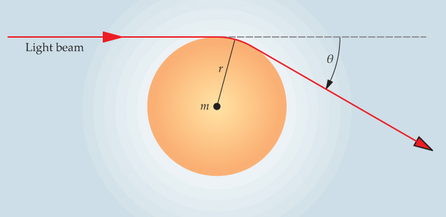
Expressed in terms of mass M, length L, and time T, the variables’ dimensions—denoted with square brackets—are [θ] = L0T0M0, [r] = L1T0M0, and [m] = L0T0M1. It follows that no combination of powers of r and m can be dimensionally homogeneous with θ.
Adding the gravitational constant G, which has dimensions L3T−2M−1, and the speed of light c, which has dimensions L1T−1M0, seems sensible for a problem concerning gravity and light. Of the potential expressions containing m, r, c, and G, algebraic calculations reveal that dimensional homogeneity is achieved only with solutions of the form mκr−κc−2κGκ, where κ is any real integer. (See reference for a step-by-step treatment.)
If the light ray skims just across the Sun’s surface, then r = 6.96 × 10⁸ m, m = 1.99 × 1030 kg, and the quantity mκr−κc−2κGκ will be small—on the order of 10−6 when κ = 1. The κ = 1 term will give the largest effect, and higher-order terms can be neglected. Arguments based purely on dimensional reasoning suggest, then, that

where α is an unknown constant. When Isaac Newton considered the problem more than 300 years ago, he arrived at an identical expression, with α = 2. General relativity predicts α = 4, and the latest experiments agree with that result to within 0.02%.
Prototypes, models, and similitude
In fluid dynamics, dimensional analysis is used to reduce a large number of parameters to a small number of dimensionless groups, often in spectacular fashion. In addition to easing analysis, that reduction of variables gives rise to new classes of similarity.
Consider the simple example of flow around a prototype airfoil, p, and a much smaller model, m, as illustrated in figure 2. The model and prototype are geometrically similar if all of their corresponding length scales, including surface roughness, are proportionate. Likewise, flows in the two systems are kinematically similar if the velocity ratios up/um are the same for all pairs of corresponding, or homologous, points.

Figure 2. A prototype airfoil (left) can be tested with a much smaller model (right), provided the objects are geometrically similar and that the flows around them are dynamically similar. Dynamic similarity is achieved if the characteristic flow velocities Up and Um are such that the forces at all homologous points—such as the two marked by asterisks—are proportionate. (Adapted from ref.
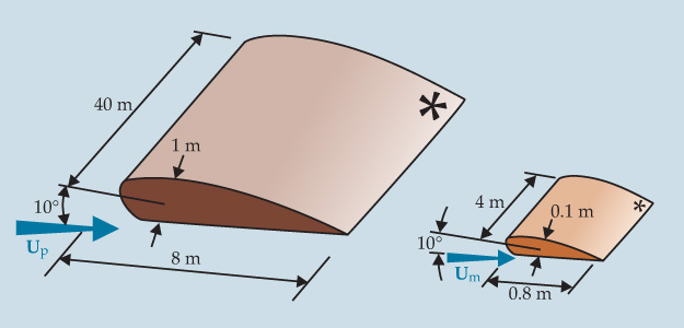
Depending on what is to be learned from the model, kinematic similarity may be too lax a requirement. The stricter standard of dynamic similarity exists if the ratios of all forces acting on homologous fluid particles and boundary surfaces in the two systems are constant. Dynamically similar systems are by definition both geometrically and kinematically similar.
An important conclusion of fluid mechanics is that incompressible, isothermal flows in or around geometrically similar bodies are considered dynamically similar if they have the same Reynolds number Re, where Re is the ratio of inertial to viscous forces (see box
If the same model were placed in a very large wind tunnel blowing air at, say, half the speed of sound, Re would be about 7 × 10⁷—closer to, but still well short of, true submarine conditions. Further options are to cool the air, thus lowering its viscosity and increasing its density—and thereby reducing the kinematic viscosity—or to operate at high pressures, increasing density more still. Adopting just that strategy, engineers at the National Transonic Facility at NASA’s Langley Research Center in Virginia reached Re of about 1 × 10⁹ in a cryogenic wind tunnel.
Cryogenic tunnels are currently among the most advanced test facilities available. Remarkably, one of the smallest such tunnels, just 1.4 cm in diameter, is capable of reaching Re as high as 1.5 million. 2
The friction factor
One consequence of dynamic similarity in pipe flows is that the so-called friction factor λ—the dimensionless shear stress exerted by the fluid on the pipe, and vice versa—is a function of Re only, provided entrance effects, surface roughness, and temperature variations are small. The friction factor is especially significant in engineering. The standard λ(Re) plot, compiled from the results of eight papers published between 1914 and 1933, is reproduced in nearly all fluid dynamics texts and spans Re from 1 × 10³ to 3 × 10⁶. Two devices exploiting two different strategies have charted new territory.
In 1998 the Princeton University team of Mark Zagarola and Alexander Smits published the first results from their “superpipe,” 3 a closed-loop, 34-m-long pipe with a nominal diameter of 12 cm. Using room-temperature air compressed as high as 187 atmospheres, the pair measured λ(Re) for Re up to 3.6 × 10⁷.
Later, a University of Oregon group led by one of us (Donnelly) designed a device consisting of a 28-cm-long pipe, roughly a half-centimeter in diameter, housed in a tabletop helium cryostat. 4 Several room-temperature gases—helium, oxygen, nitrogen, carbon dioxide, and sulfur hexafluoride—were used to measure λ(Re) for relatively small Re; liquid He was used to attain the highest Re, up to 1.1 × 10⁶.
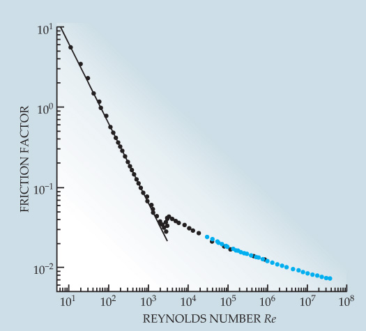
Figure 3 shows datasets from both experiments. Combined, the data span Re ranging from 11 to 37 million. Despite a dramatic difference in scale—the Princeton superpipe weighs about 25 tons, the Oregon tube about an ounce—the overlapping data sets agree 5 to within about 2%. It is a testament to the power of dynamic similarity.

Figure 3. The friction factor, the dimensionless shear stress exerted by a fluid on a pipe, is plotted as a function of the Reynolds number Re. Blue symbols correspond to data obtained from a 12-cm-wide, 34-m-long “superpipe” operated at room temperature. Black symbols correspond to data collected in a pipe roughly 1/100 000 that size, operated at cryogenic temperatures. Where they overlap, the data sets agree to within about 2%, safely within the error margin of both experiments. The solid line is the theoretical result for laminar flow, and the discontinuity near Re = 2 × 10³ corresponds to the transition to turbulence. (Adapted from ref.
Rayleigh–Bénard convection
Thermally driven convection is a conceptually simple but experimentally challenging problem. In the lab it’s typically carried out in a Bénard cell like that sketched in figure 4a, a container of fluid heated from below and cooled from above. The temperature difference ΔT gives rise to a density gradient; for typical fluids having a positive thermal expansion coefficient, the denser fluid will lie above the less dense fluid. If the density gradients are large enough, the configuration destabilizes, leading to circulating flow known as Rayleigh–Bénard convection. That convection enhances the heat transfer from the hot lower boundary to the cool upper one.
As detailed in box
The experimental challenge is to explore Nu in the highly turbulent regimes of large Ra. Dynamic similarity affords multiple ways to do so. One way to boost Ra—defined as gαL3ΔT/κν, where α, κ, and ν are the thermal expansion coefficient, the vorticity diffusivity, and the thermal diffusivity, respectively—is to create large temperature gradients. A drawback of that approach, however, is that it can yield large density variations, which complicate theoretical modeling. When ΔT is large, a central assumption of the Boussinesq equations that describe thermal convection—namely, that density depends linearly on temperature—no longer holds true (see box
Another strategy for obtaining large Ra is to use a thick fluid layer. Because Ra scales as L3, modest increases in L can produce substantial gains in Ra. Alternatively, one can choose a fluid having large α/κν. By those measures, low-temperature He is, to our knowledge, the most ideal fluid available. Extreme increases in α/κν, however, can lead to undesirably large changes in Pr.
Several experiments adopt some combination of the above strategies to explore heat transfer at the higher reaches of Ra. A University of Oregon team led by Donnelly used low-temperature He to explore Ra spanning 11 orders of magnitude. 6 Strikingly, the data, shown in red in figure 4b, are described cleanly by a single power law, with γ = 0.31.

Figure 4. Rayleigh–Bénard convection. (a) A Bénard cell consists of a layer of fluid of thickness L that’s heated from below and cooled from above. For normal fluids having a positive thermal expansion coefficient α, the configuration can be unstable—with denser fluid resting atop less dense fluid—and lead to convection. To study rotation effects, the cell can be rotated about its axis with angular velocity Ω. (b) Even in the nonrotating case, the relationship between the temperature difference T2−T1 and the heat transfer rate (shown here in dimensionless form as the Rayleigh and Nusselt numbers, respectively) remains a matter of debate. Data obtained at the University of Oregon (red), Joseph Fourier University (green), and the University of Göttingen (blue) agree at moderately large Ra, but diverge for Ra > 1013. (Data are from refs.
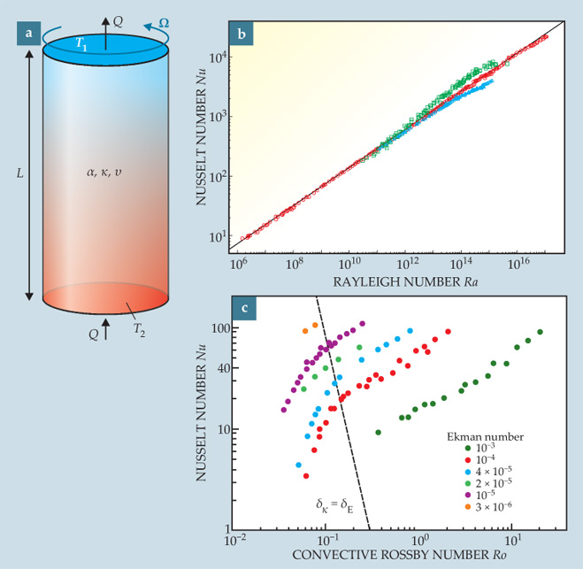
In 2001, about the same time as the Oregon data appeared, researchers at Joseph Fourier University in Grenoble, France, used a nearly identical cryogenic cell to obtain the results shown in green in figure 4b. 7 As Ra nears 2 × 10¹¹, the Grenoble data switch from a power law described by γ = 0.31 to one described by γ = 0.39. One potentially exciting interpretation is that the switch marks the transition to the “ultimate state,” a state predicted by Robert Kraichnan for asymptotically large Ra, in which the viscous boundary layers at the ends of the Bénard cell become turbulent. 8
The discrepancy between the Oregon and Grenoble data as plotted in figure 4b seems quite small. Is it of any real consequence? In geophysical and astrophysical fluid dynamics, the answer is yes. Natural phenomena such as mantle convection in Earth’s outer core, atmospheric and oceanic winds, and flows in gas giants and stars are estimated to have Ra ranging from 1020 to 1030, perhaps larger in stellar systems. Extrapolated to such geophysical and astrophysical proportions, a slight difference in scaling relationships could yield order-of-magnitude differences in Nu.
The ideas of dynamic similarity can help resolve the discrepancy. Guenter Ahlers of the University of California, Santa Barbara and colleagues at the University of Göttingen in Germany explored the range of Ra between 109 and 1015 using He, N2, and SF6 at ambient temperatures and pressures up to 15 atmospheres. 9 The high pressure, a feature absent from the Oregon and Grenoble experiments, limits changes in Pr.
Ahlers and company’s data, shown in blue in figure 4b, agree closely with the Oregon results and contradict the ultimate-state interpretation of the Grenoble data. But as the figure shows, there is still no consensus for large-Ra behavior, and the story continues to unfold. It remains unclear whether Kraichnan’s ultimate state exists, and if so, where it begins.
Rayleigh–Bénard convection, with rotation
Most convection systems of geophysical and astrophysical interest also involve rotation. The influence of rotation is studied in the lab by spinning a Bénard cell about its axis with some angular velocity Ω. Again, the flow behavior can be described in dimensionless terms. Except now, in addition to Ra and Pr, two new dimensionless numbers are also important.
The first is the convective Rossby number Ro ≡ (gαΔT/4Ω2L)1/2, the ratio of temperature-induced buoyant forces to rotation-induced Coriolis forces. One might anticipate that the transition between rotationally dominated and nonrotationally dominated flow should occur somewhere near Ro = 1.
But there is also the Ekman number E ≡ ν(2ΩL)-1, the ratio of viscous to Coriolis forces. Coriolis forces tend to sweep away the viscous boundary layer that exists near the container walls, and so the thickness δE of that boundary layer scales as E1/2. A competing length scale is the thickness δκ of the thermal boundary layer, which scales as Nu−1L. In general, communication between the container and the bulk fluid will be limited by the thinner of the two boundary layers. One might anticipate that the transition between rotationally dominated and nonrotationally dominated convection should occur when δE = δκ.
As shown in figure 4c, data from experiments at UCLA’s simulated planetary interiors laboratory confirm that the condition δE = δκ, not Ro = 1, governs the transition from rotationally dominated to nonrotationally dominated convection. 10 When δE < δκ, rotation acts to prevent convection, and heat transfer is less efficient than in a nonrotating system. When δE > δκ, rotation effects are negligible, and Nu scales as it does in the nonrotating case. With that crucial observation, the UCLA researchers were able to estimate the temperature gradients in Earth’s liquid-metal outer core as corresponding to Ra = 7 × 1024. Of course, the extrapolation of carefully controlled laboratory experiments to geophysical fluid mechanics carries caveats, several of which are detailed in reference
A real-world pendulum
Among the first problems posed to undergraduate physics students is that of a simple pendulum: a point mass suspended in a vacuum, oscillating with small amplitude. A real pendulum oscillating in a viscous fluid, however, presents a greater challenge. Wilfried Schoepe and colleagues at the University of Regensburg in Germany studied the problem 11 using a 100-µm sphere immersed in liquid He. Their data, shown in figure 5, indicate a deviation from laminar flow at a critical Re near 700.

Figure 5. A real-world pendulum.(a) At low Reynolds number Re the drag force on a spherical pendulum agrees with the Stokes prediction for laminar flow (solid line). But two experiments—one with a 100-µm sphere immersed in liquid helium (green and blue symbols), another with a 1-inch steel bob in water (red)—demonstrate that the drag force deviates from laminar flow above a critical Re near 700. Photos of the steel bob show a laminar flow structure when (b)Re < Rec and show the bob shedding vortex rings when when (c)Re > Rec. (Adapted from ref.
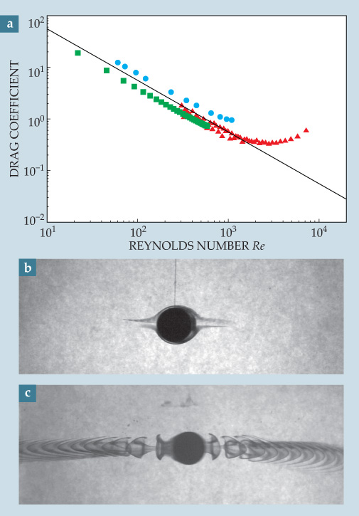
At the University of Oregon we duplicated the experiment with a 1-inch steel bob oscillating in water. The bob was 256 times as large as and 37 million times heavier than the Regensburg group’s sphere. Yet our experiment yielded a nearly identical relationship between dimensionless drag and Re and showed a similar deviation from laminar flow at large Re. Photos revealed that the steel bob starts to shed vortex rings when Re surpasses the critical value. 12
Beyond fluids
A quick check with an internet search engine reveals the ubiquity of dynamic similarity. Steven Vogel of Duke University has helped pioneer the use of dimensional analysis in biophysics. 13 He has used the concepts to highlight bounds on certain forms of physical behavior, such as the maximum height of a tree if getting sap to the leaves is the crucial factor (see PHYSICS TODAY, November 1998, page 22 ).
Principles of similarity also underlie key economic models, such as the debt-to-income ratio. For a long time now, economists have had a good understanding of what that ratio should be, regardless of total annual income, if the debt is to be manageable. A recent article, “Dimensions and Economics: Some Problems,” suggests that many commonly used models are not dimensionally homogeneous, which could result in problems during application and analysis. 14
As with all tools, it is important to be aware of the potential limitations of dynamic similarity. The principle of similarity could be crudely construed as follows: Two systems can be considered completely similar when all dimensionless numbers are the same. In practice, complete similarity is impossible to achieve unless the two systems are exactly the same.
For example, in the submarine problem, we ignored flow-compressibility effects, which become pronounced when flow speeds approach the speed of sound. Sound travels much more slowly in air than in water, so one must be cautious. It is typically assumed that as long as the flow speed is less than half that of sound, compressibility can be neglected. Similarly, Rayleigh–Bénard experiments hint that Pr, often assumed to be negligible, may play a more important role in heat transfer than once thought.
History demonstrates, however, that it is certainly possible to use principles of similarity to draw valuable parallels between systems that aren’t entirely similar. Currently, dynamic similarity and dimensional analysis are topics that engineering students learn as part of their fluid mechanics course, typically in the second or third undergraduate year. We believe that emphasis on dimensional reasoning would be useful to students in many branches of physics as well.
Box 1. A brief history of dimensional analysis
Going back more than 300 years, discussions of dimensional analysis have appeared in scores of texts, often with different slants:
1687. Isaac Newton publishes the Principia, which, in book II, section 7, contains perhaps the earliest documented discussion of dimensional analysis.
1765. Leonhard Euler writes extensively about units and dimensional reasoning in Theoria motus corporum solidorum seu rigidorum, a comprehensive treatment of the mechanics of rigid bodies.
1822. Joseph Fourier employs concepts of dimensional analysis in his Analytical Theory of Heat.
1877. Lord Rayleigh outlines a “method of dimensions” in his Theory of Sound.
1908. At the 4th International Congress of Mathematicians in Rome, Arnold Sommerfeld introduces a dimensionless number that he calls the Reynolds number, in tribute to Osborne Reynolds. The Reynolds number, which appeared in what’s now known as the Orr–Sommerfeld equation, is among the most famous of all dimensionless numbers.
1914. In what is generally regarded as the big breakthrough in dimensional analysis, physicist Edgar Buckingham introduces the theorem now known as the Buckingham Pi theorem. It is one of several methods of reducing a number of dimensional variables to a smaller number of dimensionless groups.
1922. In his influential book Dimensional Analysis, Percy Bridgman outlines a general theory of the subject.
1953. In his George Darwin lecture before the Royal Astronomical Society, Subrahmanyan Chandrasekhar names the Rayleigh number, a dimensionless temperature difference central to thermal convection.
Box 2. The origins of some dimensionless numbers in fluid mechanics
The Reynolds number. The most famous of the dimensionless numbers, the Reynolds number, can be derived from the Navier–Stokes equations for incompressible flows:

where u is local velocity, p is pressure, ρ is the fluid density, and ν is the fluid’s kinematic viscosity.
Choosing appropriate characteristic length and velocity scales, L and U, one can introduce a dimensionless displacement x′ ≡ x/L, dimensionless time t′ ≡ tU/L, dimensionless velocity u′ ≡ u/U, and dimensionless pressure p′ ≡ p/ρU2. The Navier–Stokes equations become

where Re = UL/ν is the Reynolds number.
The change to dimensionless variables is not just a superficial step; it greatly reduces the amount of work needed to study a given flow. Although it might seem that one would need to investigate separately the effects of varying ρ, L, U and ν, one needs to investigate only variations with Re.
The Rayleigh, Prandtl, and Nusselt numbers. Assuming density variations are small, thermal convection can be described by the Boussinesq equations,

where α and κ are, respectively, the fluid’s thermal expansion coefficient and thermal diffusivity, g is the acceleration due to gravity, and T is temperature. Nondimensionalization of the Boussinesq equations yields two key parameters: the Rayleigh number Ra ≡ gαL/κν, the dimensionless temperature difference, and the Prandtl number Pr ≡ ν/κ, the ratio of vorticity diffusivity to thermal diffusivity.
The heat transfer rate is usually described in terms of the Nusselt number Nu, the ratio of the actual heat transfer Q to the heat transfer Qc that would result from conduction alone. For nonrotating Bénard cells having the same shape and boundary conditions, Nu is completely determined by Ra and Pr.
The authors are grateful to Guenter Ahlers, Jonathan Aurnou, Paul Roberts, Alexander Smits, Edward Spiegel, and Katepalli Sreenivasan for their useful suggestions.
References
1. R. Kurth, Dimensional Analysis and Group Theory in AstrophysicsPergamon Press, Oxford, UK (1972).
2. C. Swanson, R. J. Donnelly, in Flow at Ultra-High Reynolds and Rayleigh Numbers: A Status ReportR. J. Donnelly, K. Sreenivasan, eds.,Springer, New York (1998), p. 206.
3. M. V. Zagarola, A. J. Smits, J. Fluid Mech. 373, 33 (1998). https://doi.org/10.1017/S0022112098002419
4. C. J. Swanson, B. Julian, G. G. Ihas, R. J. Donnelly, J. Fluid Mech. 461, 51 (2002).
5. B. J. McKeon, C. J. Swanson, M. V. Zagarola, R. J. Donnelly, A. J. Smits, J. Fluid Mech. 511, 41 (2004). https://doi.org/10.1017/S0022112004009796
6. J. J. Niemela, L. Skrbek, K. R. Sreenivasan, R. J. Donnelly, Nature 404, 837 (2000).
Data revised slightly in J. J. Niemela, K. R. Sreenivasan, J. Low Temp. Phys. 143, 163 (2006). https://doi.org/10.1007/s10909-006-9221-97. X. Chavanne, F. Chillà, B. Chabaud, B. Castaing, B. Hébral, Phys. Fluids 13, 1300 (2001). https://doi.org/10.1063/1.1355683
8. R. Kraichnan, Phys. Fluids 5, 1374 (1962). https://doi.org/10.1063/1.1706533
9. D. Funfschilling, E. Bodenschatz, G. Ahlers, Phys. Rev. Lett. 103, 014503 (2009); https://doi.org/10.1103/PhysRevLett.103.014503
G. Ahlers, D. Funfschilling, E. Bodenschatz, New J. Phys. 11, 123001 (2009). https://doi.org/10.1088/1367-2630/11/12/12300110. E. M. King, S. Stellmach, J. Noir, U. Hansen, J. M. Aurnou, Nature 457, 301 (2009); https://doi.org/10.1038/nature07647
E. M. King, K. M. Soderlund, U. R. Christensen, J. Wicht, J. M. Aurnou, Geochem. Geophys. Geosyst. 11, Q06016 (2010), doi:https://doi.org/10.1029/2010GC003053 .11. J. Jäger, B. Schuderer, W. Schoepe, Physica B 210, 201 (1995). https://doi.org/10.1016/0921-4526(94)01108-D
12. D. Bolster, R. E. Hershberger, R. J. Donnelly, Phys. Rev. E 81, 046317 (2010). https://doi.org/10.1103/PhysRevE.81.046317
13. S. Vogel, J. Biosci. 29, 391 (2004) https://doi.org/10.1007/BF02712110 ;
30, 167 (2005);
30, 303 (2005);
30, 449 (2005);
30, 581 (2005).14. W. Barnett, Q. J. Austrian Econ. 7, 95 (2004).
15. F. M. White, Fluid Mechanics McGraw-Hill, New York (1994), p. 276.
More about the authors
Diogo Bolster is an assistant professor of civil engineering and geological sciences at the University of Notre Dame in Notre Dame, Indiana. Robert Hershberger is a research assistant in the department of physics at the University of Oregon in Eugene. Russell Donnelly is a professor of physics at the University of Oregon.


