Beyond quantum jumps: Blinking nanoscale light emitters

Imagine driving your car at night while its headlights display an annoying blinking behavior, switching on and off randomly. To add to the nuisance, the blinking has no definite time scale. In fact, although in most of your nightly journeys your headlights display quite rapid blinking, rendering at least some visibility, occasionally they remain off for almost the entire journey.

Ridiculous and impractical as that behavior may seem, such is the situation commonly encountered by nanoscientists: A wide variety of natural and artificial nanoscopic light emitters, from fluorescent proteins to semiconductor nanostructures, display a blinking behavior like that described above. The emission (on) and no-emission (off) periods have a duration that varies from less than a millisecond to several minutes and more. The probability of occurrence of the on and off times is characterized by a power law, which is a typical sign of high complexity and is fundamentally different from what is expected from the quantum jump mechanism of fluorescence blinking predicted at the dawn of quantum mechanics.

So what is the origin of the power-law blinking? Since it is a nearly universal behavior of single emitters, we tend to think there must be a fundamental answer. Remarkably, even a decade after the behavior was discovered, a satisfactory explanation of the power-law blinking has managed to evade all the experimental and theoretical efforts. That enigmatic luminescence blinking and its peculiar statistical consequences are the focus of this article.

Quantum jumps and fluorescence blinking

Almost a century ago, Niels Bohr proposed his now famous model in which electrons occupy discrete energy levels, or orbits, within the atom. That energy discretization led Bohr to the “quantum jump” prediction: Since electrons cannot be between states, they must undertake instantaneous leaps from one state to another. Direct experimental observation of quantum jumps had to wait until the mid-1980s, when individual ions could be trapped and addressed optically. The jumps were detected as interruptions in the fluorescence emission of single ions when a second electronic transition from a common ground or excited state was pumped in parallel (see box 1 on page 35). Later, in the early 1990s, experiments on single fluorescent molecules again revealed the occurrence of quantum jumps as interruptions of the fluorescence signal, this time due to weak transitions from the excited state to a long-lived triplet state (see box 1). Such fluorescence blinking has since become a hallmark of single quantum emitters.

The breakthrough of single-molecule detection brought unprecedented detail into many areas of physics and led to the discovery of numerous surprising effects. Individual nanoscale emitters can be used as fluorescent markers for a number of physical and chemical processes. By attaching them to large biomolecules, for instance, one can directly observe conformational changes and molecular function. Furthermore, one may follow trajectories of individual molecules and thereby track dynamics in a biological cell, for example. The great potential of single-molecule measurements is often restricted by two phenomena. The first one is obviously the blinking: If it occurs on a time scale relevant to the experiment, it complicates the retrieval of information. Second, measurements are limited by photobleaching: Excited molecules may use their excess energy to undergo irreversible chemical reactions that render them nonfluorescent.

Power-law blinking

Studies of the long time scales of blinking events had to await the construction of bleaching-resistant emitters. Those nanoscopic light sources, enabling virtually infinite measurement times, were semiconductor nanocrystals, commonly referred to as colloidal quantum dots. Described in box 2 on page 36, QDs are one of the most prominent examples of nanotechnology due to their fascinating size-dependent electronic and optical properties. ¹

Fluorescence blinking of individual QDs was first observed in 1996 by a collaboration between the groups of Moungi Bawendi at MIT and Louis Brus, then at Bell Laboratories. ² Actually, it was surprising to find QD blinking at all because no mechanism known at the time would affect a dot’s emission. Adding to the surprise, the researchers immediately realized that the sojourn times—the times spent in the on and off states—were not exponentially distributed, a result that implied the presence of complex processes behind the new blinking phenomenon. Later, Masaru Kuno, David Nesbitt, and coworkers at JILA found that the probabilities of the on and off times follow a power law (see figure 1) of the form

$$\begin{array}{cc}P\left(t\right)\propto t^{-\alpha },& 1<\alpha <2,\end{array}$$ ((1))

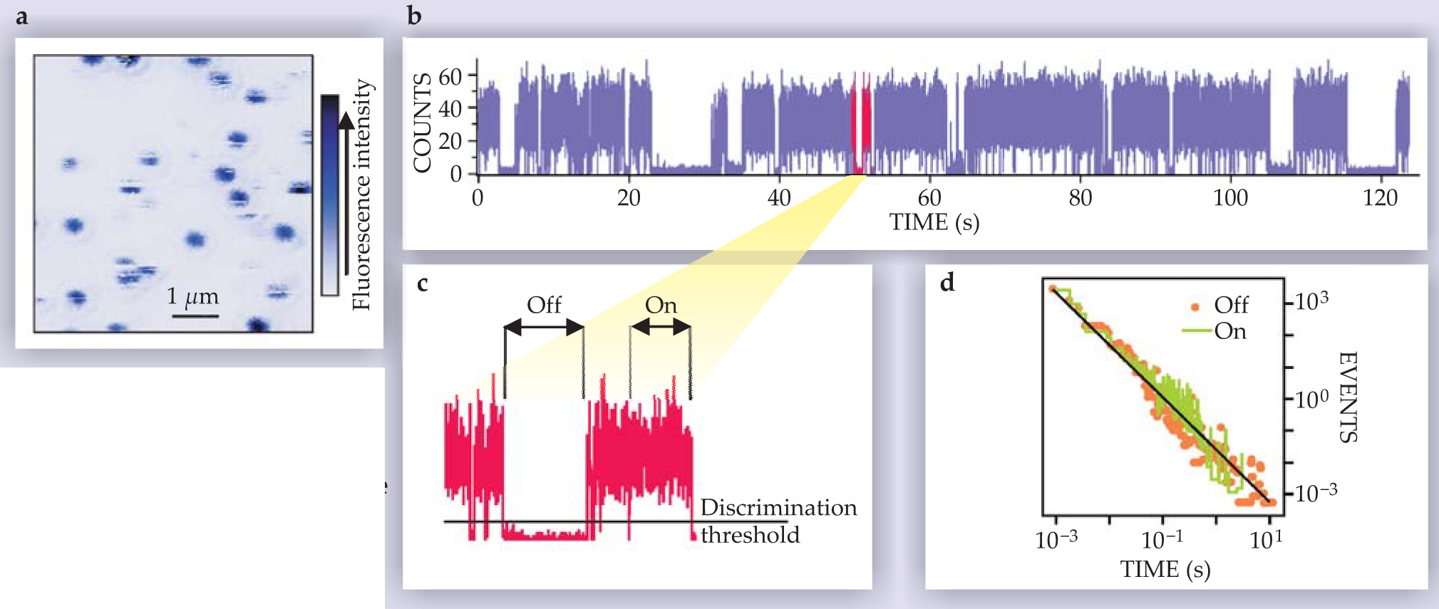
where t is the length of the on or off sojourn time and the exponent α lies between 1 and 2 (typically close to 1.5). ³

The emission of single colloidal QDs can be monitored for hours, and the on and off times have a power-law distribution over several decades in time. Further experimentation showed that all colloidal QDs display the same kind of behavior, regardless of their size, composition, and structure—whether the QD consisted of a bare semiconductor core or of a core surrounded by an inorganic shell. Although an accurate determination of α is not trivial, some studies indicate that the on- and off-state exponents are identical and that they are independent of temperature and of the intensity of the exciting light source. Yet when the intensity is strong enough, exponential cutoffs of the distributions of the sojourn times are observed, usually leading to shorter maximum on times than off times. ⁴

In recent years different routes to circumvent photobleaching in other systems led to the discovery that power-law blinking is not exclusive to QDs. ⁵ The same power-law blinking has been uncovered in almost any type of single quantum emitter embedded in a disordered medium, including semiconductor nanorods and longer nanowires, organic molecules, fluorescent proteins, and conjugated polymers.

Statistical effects

The main property of power laws is their scale invariance. It can be seen from equation (1) that scaling the times by a constant factor c causes only proportional scaling of the whole function: P(ct) ∝ P(t). Variables with a power-law distribution have been observed in a wide variety of situations and are usually indicative of highly complex processes. Examples include the Gutenberg–Richter law for the distribution of earthquake sizes, scaling laws in biological systems (see the article by Geoffrey West and Jim Brown in Physics Today, September 2004, page 36 ), the degree of links in social and physical networks (see the article by Mark Newman in Physics Today, November 2008, page 33 ), and Pareto’s law of income distribution (see the article by Doyne Farmer, Martin Shubik, and Eric Smith in Physics Today, September 2005, page 37 ). In physics, scale invariance is observed in critical phenomena: Many physical quantities, such as heat capacity or compressibility display a power-law dependence on temperature near the critical point. Other examples are found in charge transport and diffusion in disordered media like amorphous semiconductors, glasses, and liquids (see the article by Harvey Scher, Michael Shlesinger, and John Bendler in Physics Today, January 1991, page 26 ) and chaotic dynamics in deterministic systems (see the article by Joseph Klafter, Michael Shlesinger, and Gert Zumofen in Physics Today, February 1996, page 33 ).

It is evident from equation (1) that ∫ ₀ ^∞ t P(t)dt = ∞. Thus the average on and off times diverge! That makes for a rather uncomfortable situation in physics, since it is a common practice to try to identify the inherent scale of a problem. However, systems described by power laws don’t have a characteristic scale. Interestingly unlike previous examples of scale-free processes, blinking single emitters exhibit that behavior at the single-particle level, which leads to what is called weak ergodicity breaking. ⁶ In practice, ergodicity means that time averages are equal to ensemble averages. Ergodicity is the foundation on which statistical mechanics is built, and it is often assumed to be valid when the time traces of signals are analyzed.

Imagine an experiment in which we collect the light emitted by an ideal QD under continuous excitation. For simplicity assume the sojourn times in the on and off states are identically distributed with a probability given by equation (1). When the dot is in the on state, the intensity I of emitted light is I ₀, and when it is in the off state, the intensity is zero. Imagine now that we take many such dots and measure the emission intensity. Clearly, due to the assumed symmetry between on and off states, the ensemble average intensity 〈I〉 = I ₀/2. Now consider the time-averaged intensity Ī emitted by one individual dot in a period of length T:

$$\overline{I}=\frac{{\int }_0^{T}I\left(t\right)dt}{T}=I_0\times \frac{Totaltimeintheonstate}{T}$$.((2))

If an average sojourn time exists, as it does when the distribution of sojourn times is exponential, and we make the measurement time T long enough, we would find the usual ergodic result that Ī = 〈I〉. However, if the time scale of the problem is infinite, as is the case with the power law of equation (1), we can never time-average long enough to obtain ergodicity. Instead, in some cases the dot is found in the on state (or the off state) for periods that are of the order of the measurement time, in which case the time-averaged intensity will be close to I ₀ (or to zero). In other words, repeated measurements of time-averaged intensity on the same QD, under the same physical conditions, do not yield a reproducible result! Such randomness is, in fact, inherent. Stochasticity, of course, is not new, but in the situation we are addressing here, the long time average itself is a random variable. In the case of power laws, the ergodicity breaking is called weak because the QDs do explore their state space—each individual dot will jump many times between the two states, on and off. Strong ergodicity breaking would mean that some of the dots remain always in the on state, while others are always in the off state. For more on the ergodicity breaking of QD blinking, see box 3 on page 38.

Physical mechanisms

What could be the physical process behind the fluorescence intermittency? Most of the proposed blinking mechanisms are inspired by work done in the late 1980s by Alexander Ekimov, Alexander Efros, and coworkers at the Ioffe Institute in Saint Petersburg, who examined cadmium sulfide nanocrystals embedded in glass matrices. ⁷ Those nanocrystals were the first that showed size-dependent quantum effects. In that system, Ekimov and colleagues found that electrons from excited QDs could escape from the dot into long-lived trap states in the glass. Furthermore, they observed that the luminescence of an ensemble of CdS QDs decreased with time under constant illumination. That “photodarkening” was explained by a mechanism called photoassisted Auger ionization, which accounted for all experimental observations: A doubly excited QD could expel an electron out of the dot by using the recombination energy of one of the excitons. The lone hole left in the dot rapidly takes up the energy of subsequently generated excitons and thus provides a fast, non-radiative relaxation pathway and reduced luminescence.

Soon after the observation of luminescence blinking of single QDs, Efros and Mervine Rosen at the US Naval Research Laboratory suggested the first possible explanation based on the above picture: the direct manifestation of the dynamics of photoassisted Auger ionization. ⁸ An off period starts when an electron is expelled from the QD, and it ends once the electron returns via a tunneling or thermally activated process (figure 2(a)). Within that picture, the blinking sequence on → off → on … corresponds to neutral dot → charged dot → neutral dot…. Although that model would explain why blinking occurs in QDs, it does not predict the power-law distributions of on and off times. Further, the requirement of a doubly excited QD suggests a quadratic dependence on the excitation intensity for the switching-off process, but such a dependence is not observed in the experiments. Still, the physical picture is intuitive and sensible, and different mechanisms for the ionization and neutralization of QDs have been investigated theoretically in efforts to account for the experimental observations. ⁹

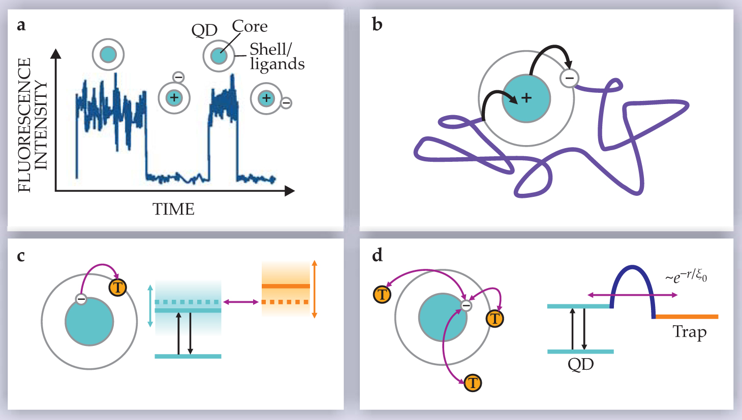
Probably the simplest possibility is to consider that once the electron leaves the QD (such as by the photoassisted Auger process), it may diffuse in the vicinity of the QD before it returns (figure 2(b)). But if the electron can diffuse freely, it has a finite probability of escaping to infinity. That is related to a well-known theorem of George PöAlya: The probability is one for a random walker to return to the origin in one or two dimensions, but it is less than one in three or more dimensions. Therefore, after some on–off cycles, the QD would remain off forever, simply because the electron escaped to infinity. However, when the electron is ejected to the surrounding matrix, the dot remains positively charged. Due to the Coulomb attraction, the electron cannot diffuse freely. Indeed, at room temperature the thermal energy is smaller than the Coulomb interaction energy within a distance of roughly 7 nm, which is larger than the typical dot size. Therefore, the escape probability is significantly reduced. In a model in which the electron is allowed to both diffuse and hop back to the dot from the matrix, either by tunneling or thermal activation, the probability of escape is zero and the power-law exponent α, though dependent on parameters of the model, varies around α = 3/2. The deviations can be small when diffusion is the main contributor to the electron’s return to the dot.

Instead of diffusion in space, we may consider a “diffusion” of energy levels as suggested by Bawendi and coworkers at MIT. The idea is that electrons may escape from the dot and return to it via resonant tunneling between an excited state in the QD and a trap state, located outside the QD or at the surface (figure 2(c)). Then, switching between the on and the off states occurs only when the energy levels of the QD and the trap match. If we let an energy level diffuse, it may stay close to the resonant energy and perform many crosses (providing many chances to switch on or off), but it also may drift very far and take a long time to return to resonance. If the energy levels fluctuate randomly, one can use simple one-dimensional random-walk theory to calculate the probability density function, which naturally leads to a power-law probability of on and off times with α = 3/2.

An alternative tunneling mechanism to explain the power-law blinking was suggested by Kuno and coworkers at JILA and by Michel Orrit’s group at the University of Leiden. Here again, an excited electron in the QD may tunnel to a trap site, presumably located on the surface of the capping shell or in the disordered matrix in the vicinity of the dot (figure 2(d)). The off time is then determined by the recovery time of the electron, which for a tunneling mechanism is given by τ = τ₀ e ^r/ξ₀ , where 1/τ₀ is an attempt frequency r is the distance between the QD and the trap, and ξ₀ is a length scale that can be obtained using the Wentzel-Kramers-Brillouin (WKB) theory. The off-time expression reflects that the further the trap is from the dot, the longer the recovery time. More importantly, τ depends exponentially on r, which means that small changes in r may induce large changes in τ. In the vicinity of the dot there are many traps, and each time an electron is ejected from the dot it will randomly choose one of those traps. If the traps are randomly located with an exponential distribution f(r) = 1/ξ₁ e ^−r/ξ₁ , one finds by change of variables that the probability density function of the off times is given by a power law with exponent α = 1 + ξ₀/ξ₁. Thus α is related to the two exponential length scales of the problem: ξ₁ describes the disorder of the relevant traps and ξ₀ gives the scale for exponential sensitivity of τ on r. It is reasonable to assume that the scales and hence α are not sensitive to temperature and, unlike the diffusion models, α is not necessarily fixed to 3/2. The main lesson to learn from this approach, sometimes called the exponential conspiracy is that a simple transformation of standard random variables, with well-defined averages, may lead to power-law kinetics.

More puzzles

Each of the above theoretical frameworks has succeeded in explaining some of the characteristics of power-law blinking, but never all of them. For instance, a considerable number of research groups have reported exponents deviating from the α = 3/2 predicted by the diffusion models. The different exponents, which in some cases are found to depend on the environment, could be accounted for by the electron-tunneling model with a distribution of trap states, which also naturally accounts for the insensitivity of power-law blinking kinetics to temperature. However, that model fails to explain the power-law distribution of on times, which follows rather straightforwardly from the energy-level diffusion model. In addition, some observations can’t be explained satisfactorily by any of the models in their present form. For example, a memory effect has recently been uncovered in the distributions of both the on and the off times: A long on time is followed with higher probability by another long on time. ¹⁰ The same happens with successive off times, but curiously it does not happen for consecutive on and off times, which hints that the two processes might be independent.

All in all, some experiments have raised more questions than they answered, and conclusive experiments still have to be done. For example, the dependencies of the blinking on the wavelength and intensity of the pump light source, and the effects of external electric and magnetic fields, still need to be thoroughly explored. Given the generally high complexity of which a power-law distribution is reminiscent, it might well be that a combination of various mechanisms is at play. Additionally, theoretical approaches that do not consider QD charging have been hypothesized, ¹¹ but it remains to be seen whether such alternatives will lead to increased insight.

Despite our lack of understanding of how the power-law behavior actually arises, two approaches to influence the blinking have recently been developed. First, in attempts to functionalize QDs for different applications, various ligand molecules have been used to modify the QD surface, and they turn out to have a strong influence on the photophysical behavior. ¹² For example, electron-donating ligands lead to a drastic reduction in the length and frequency of the off times. However, the blinking kinetics do not necessarily change concomitantly; although off times occur less frequently, they still follow a power-law distribution. Thus, while an important step for practical applications has been made in reducing the frequency of unwanted blinking events, it remains to be seen what that approach can bring to our understanding of how the power-law behavior arises.

In a second approach, blinking has been suppressed by synthesizing QDs with a core of CdSe QDs surrounded by thick (5–15 nm) shells of highly crystalline CdS. ¹³ Such findings add to the notion that the power-law blinking is related to a disordered environment and does not arise in a crystalline medium. In fact, it was already known that so-called self-assembled QDs, which under certain conditions spontaneously form during epitaxial growth of high-quality crystals and have a nearly perfect lattice match with the embedding material, do not show fluorescence blinking.

A nonblinking nanoscopic light emitter will be an important breakthrough for practical applications. That the blinking behavior can be influenced by surface modifications makes us think the first steps to achieve that goal have been made. However, that’s not certain. The origin of power-law blinking remains unknown, and as we have seen here, taking random steps can make us spend very long times on the wrong side of where we want to be. Some things are clear: Both the QD structure and its immediate nano-environment play crucial roles. And from the viewpoint of a physicist, it is fascinating to find such rich behavior in a system as small as a nano-sized single emitter and to be challenged to unravel its mechanism.

References

1. A. P. Alivisatos, Science 271, 933 (1996). https://doi.org/10.1126/science.271.5251.933
2. M. Nirmal, B. O. Dabbousi, M. G. Bawendi, J. J. Macklin, J. K. Trautman, T. D. Harris, L. E. Brus, Nature 383, 802 (1996). https://doi.org/10.1038/383802a0
3. M. Kuno, D. P. Fromm, H. F. Hamann, A. Gallagher, D. J. Nesbitt, J. Chem. Phys. 115, 1028 (2001). https://doi.org/10.1063/1.1377883
4. K. T. Shimizu, R. G. Neuhauser, C. A. Leatherdale, S. A. Empedocles, W. K. Woo, M. G. Bawendi, Phys. Rev. B 63, 205316 (2001); https://doi.org/10.1103/PhysRevB.63.205316
F. D. Stefani, W. Knoll, M. Kreiter, X. Zhong, M. Y. Han, Phys. Rev. B 72, 125304 (2005). https://doi.org/10.1103/PhysRevB.72.1253045. J. P. Hoogenboom, E. M. H. P. van Dijk, J. Hernando, N. F. van Hulst, M. F. García-Parajó, Phys. Rev. Lett. 95, 097401 (2005); https://doi.org/10.1103/PhysRevLett.95.097401
R. Zondervan, F. Kulzer, S. B. Orlinskii, M. Orrit, J. Phys. Chem. A 107, 6770 (2003). https://doi.org/10.1021/jp034723r6. X. Brokmann, J. -P. Hermier, G Messin, P. Desbiolles, J. -P. Bouchaud, M. Dahan, Phys. Rev. Lett. 90, 120601 (2003); https://doi.org/10.1103/PhysRevLett.90.120601
G. Margolin, E. Barkai, Phys. Rev. Lett. 94, 080601 (2005). https://doi.org/10.1103/PhysRevLett.94.0806017. A. I. Ekimov, A. L. Efros, Phys. Status Solidi B 150, 627 (1988); https://doi.org/10.1002/pssb.2221500244
D. I. Chepic, A. L. Efros, A. I. Ekimov, M. G. Ivanov, V. A. Kharchenko, I. A. Kudriavtsev, T. V. Yazeva, J. Lumin. 47, 113 (1990). https://doi.org/10.1016/0022-2313(90)90007-X8. A. L. Efros, M. Rosen, Phys. Rev. Lett. 78, 1110 (1997). https://doi.org/10.1103/PhysRevLett.78.1110
9. P. Frantsuzov, M. Kuno, B. Jankó, R. A. Marcus, Nat. Phys. 4, 519 (2008); https://doi.org/10.1038/nphys1001
F. Cichos, C. von Borczyskowski, M. Orrit, Curr. Opin. Colloid Interface Sci. 12, 272 (2007); https://doi.org/10.1016/j.cocis.2007.07.012
G. Margolin, V. Protasenko, M. Kuno, E. Barkai, Adv. Chem. Phys. 133, 327 (2006).10. F. D. Stefani, X. Zhong, W. Knoll, M. Han, M. Kreiter, New J. Phys. 7, 197 (2005); https://doi.org/10.1088/1367-2630/7/1/197
J. P. Hoogenboom, J. Hernando, M. F. García-Parajó, N. F. van Hulst, J. Phys. Chem. C 112, 3417 (2008). https://doi.org/10.1021/jp710100b11. P. A. Frantsuzov, R. A. Marcus, Phys. Rev. B 72, 155321 (2005). https://doi.org/10.1103/PhysRevB.72.155321
12. V. Fomenko, D. J. Nesbitt, Nano Lett. 8, 287 (2008). https://doi.org/10.1021/nl0726609
13. B. Mahler, P. Spinicelli, S. Buil, X. Quelin, J.-P. Hermier, B. Dubertret, Nat. Mater. 7, 659 (2008); https://doi.org/10.1038/nmat2222
Y. Chen, J. Vela, H. Htoon, J. L. Casson, D. J. Werder, D. A. Bussian, V. I. Klimov, J. A. Hollingsworth, J. Am. Chem. Soc. 130, 5026 (2008). https://doi.org/10.1021/ja711379k
More about the authors
Fernando Stefani is a group leader in the department of physics at the Ludwig Maximilian University of Munich and the Center for NanoScience in Munich, Germany. Jacob Hoogenboom is an assistant professor of applied physics at Delft University of Technology in the Netherlands. Eli Barkai is a professor of physics at Barllan University in Ramat Gan, Israel, and a visiting scientist at the Massachusetts Institute of Technology in Cambridge.
Fernando D. Stefani, 1 Ludwig Maximilian University of Munich and the Center for NanoScience in Munich, Germany .
Jacob P. Hoogenboom, 2 Delft University of Technology, Netherlands .
Eli Barkai, 3 Bar-Ilan University in Ramat Gan, Israel .