Back to the beginning of quantum spacetime
DOI: 10.1063/PT.3.1916
If there was no birth-time of earth and heaven and they have been from everlasting, why before the Theban war and the destruction of Troy have not other poets as well sung other themes?
—Lucretius, De rerum natura
If there was no birth-time of earth and heaven and they have been from everlasting, why before the Theban war and the destruction of Troy have not other poets as well sung other themes?
—Lucretius, De rerum natura
Ever since our distant ancestors began to contemplate the world around them, the question of its beginning has been on humankind’s mind. The above quotation, from Lucretius’s first-century-BCE work De rerum natura, can be found in the treatise The Birth-Time of the World, published in 1914 by John Joly, a professor of geology at Trinity College Dublin. True to his profession, Joly moves the realm of first events from cultural achievements and mischief to the impersonal planet Earth. He writes: “Notwithstanding our limitations, the date of the birth-time of our geological era is the most important date in Science.”
Interest in the question of how it all began has persisted throughout the millennia, but our understanding of what “all” sums up has evolved. Scientific discoveries have led us to push the beginning back to earlier and earlier times, and nowadays, following the advent and great success of modern cosmology, we tend to disagree with Joly and shift the beginning to grander cosmic events. Physicists have developed theories about the formation of galaxies and the stars they contain, the nucleosynthesis of elements, the genesis of protons and neutrons from quarks, and more speculatively, the creation of matter excitations during cosmic inflation from nothing but quantum fluctuations.
Exciting matter out of the vacuum seems to violate energy conservation, and indeed, conservation laws are the strictest keepers of the gates of time: If some quantities must remain constant, they cannot begin to acquire nonzero values. At whatever time we choose to mark “the beginning,” conserved quantities must remain zero, exactly balanced. In theory, inflation can produce matter energy, but only by taking it from some other source—spacetime. According to general relativity, the energy-balance law includes not only the usual matter terms but also a negative contribution from spacetime. The sum always remains zero, and matter can arise.
If matter forms under gravity’s sponsorship, it cannot be part of the absolute beginning. Yet again, we have to push the beginning backwards. Matter emerges from spacetime, but how did space and time begin? How can it even be possible that time had an absolute beginning, with no time “before”?
The physicality of time and space
Spacetime is dynamical, affects matter, and is in turn influenced by matter, obeying Einstein’s equation of general relativity. As a dynamical entity, it could have had a beginning, according to a scenario commonly associated with the Big Bang model. Indeed, many solutions of Einstein’s equation show an ever-expanding cosmos, starting at zero size. At zero size, however, Einstein’s equation breaks down; some expressions in the differential equation diverge. A universe of zero size, the Big Bang singularity, is not the beginning of spacetime but a limitation of the theory. General relativity simply does not address what might have been before the Big Bang. It does not tell us there was nothing.
Quantum theory should provide a better grasp, perhaps even of the beginning. We physicists are familiar with the creation of particles out of the vacuum. Quantum physics should also apply to spacetime, a dynamical and physical object in its own right. But problems loom. For instance, would a quantum theory of spacetime need to include fluctuations of time or temporal superpositions? When Charles Dickens wrote in A Christmas Carol, “the figure itself fluctuated in its distinctness: being now a thing with one arm, now with one leg, now with twenty legs, now a pair of legs without a head, now a head without a body,” he envisioned the number of limbs to fluctuate, but time for him kept ticking at regular beats of “now.” Quantum-gravity theorists still struggle with the notion of fluctuating time.
Quantum mechanics implies atomic building blocks. It remains unclear what the elementary constituents of spacetime are or what their absence would mean. Empty space, the vacuum free of matter excitations, is not empty, for there is still space. The vacuum of quantum gravity, devoid even of spacetime excitations, would be emptier than empty space. We are reaching the limits of logic and language, and those limitations are a prelude to the conceptual difficulties faced in quantum gravity.
Dimensional arguments provide estimates for the microscopic scale of spacetime. Newton’s constant G, Planck’s constant ℏ, and the speed of light c give a unique length parameter, the tiny Planck length ℓP = √
Those scales do not give much hope for experimental tests. Indeed, the scientific community’s observational abilities are far from being able to resolve the Planck length scale of spacetime atoms and will remain so for decades or more to come. Observations on large scales are one possible way out; perhaps microscopic properties will manifest themselves in many-body phenomena, as they do in condensed-matter physics.
Moreover, dimensional arguments can and usually do fail for systems described by large dimensionless numbers or by two or more parameters of the same dimension. For example, one can guess the Bohr radius of a hydrogen atom, r0 = 4πε0ℏ2/(e2me), by combining the relevant constants of nature. But atoms of high atomic number Z are more complicated. To decide whether the radius is Zr0, r0/Z, or some other function requires a knowledge of the physics involved. Similarly, to see the relevance of the Planck scale, cosmologists will need a good quantum theory of spacetime. One candidate is loop quantum gravity, which aims to promote classical relativistic structures to the quantum level and has led to concrete and encouraging examples for understanding the physical role of the Planck scales. One structure of particular interest, the subject of the following section, is called the hypersurface-deformation algebra; it is the mathematical form that relates different orderings of perturbations to spatial surfaces.
Deform, wait, deform back
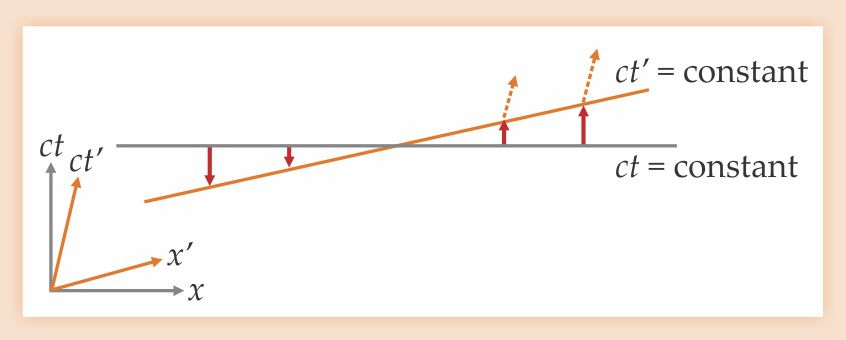
In the Minkowski space of special relativity, constant-time surfaces as experienced by different inertial observers are related by linear deformations. For example, as illustrated in figure 1, the surface identified by a moving (boosted) observer as time t′ = 0 can be expressed as a deformation T(N) of the t = 0 surface of a stationary observer; the recipe is to displace every point x on the stationary observer’s surface by the appropriate distance N(x) in the normal direction. If we boost to velocity v, wait for some time Δt, and then apply the reverse boost, all objects move a distance Δx = vΔt. Figure 2 gives a perhaps surprising geometrical interpretation of that result.

Figure 2. An object shifts position if it is boosted to velocity v, it moves around for a time Δt, and then it is returned to its original stationary state. These diagrams give a geometric representation of that simple result for v ≪ c. The upper illustration shows the normal deformation N1(x) = vx/c followed by a second normal deformation N2(x) = cΔt − vx/c. In the bottom illustration, the deformations are carried out in the reverse order. In both cases, a constant-t surface is ultimately transformed to a constant-t surface; the difference between the two composite transformations gives the shift Δx (blue arrows). Because all the slanted red arrows in the figure make an angle of tan−1(v/c) with the vertical, one can readily confirm that Δx = vΔt, the correct law for inertial motion.
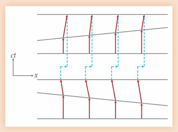

Figure 1. A Lorentz boost, which changes an observer’s velocity, implies a transformation of constant-time spatial slices of spacetime. The t′ = 0 surface of a boosted observer is related to the t = 0 surface of the stationary observer by a linear deformation T(N): Each point x on the t = 0 surface is shifted by a distance N(x) = vx/c along the normal direction. Note that normal vectors are drawn according to Minkowski geometry, parallel to the time axes, so a subsequent boost would involve deformations in the direction indicated by the orange, dotted arrows.
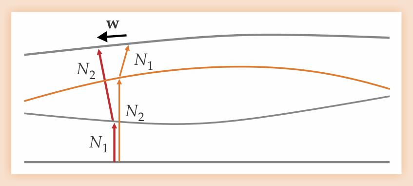
General relativity provides transformation laws for nonlinear coordinate changes—in particular, nonlinear N(x)—which imply arbitrary deformations of space. Relations, such as illustrated in figure 3, between different deformations lead to the hypersurface-deformation algebra. Its most important part generalizes the geometric result depicted in figure 2: Two time deformations T(N) performed in opposite orderings differ by a spatial displacement S(w),

Figure 3. General relativity allows for nonlinear coordinate changes, which correspond to arbitrary deformations S(w) within spatial slices and arbitrary temporal deformations T(N), with functions N determining the shift along the normal at every point. The example shown here generalizes figure
T(N2)T(N1) − T(N1)T(N2) = S(N2∇N1 − N1∇N2). (1)
For the two linear functions N1 and N2 introduced in figure 2, equation 1 reduces to Δx = vΔt.
General relativity embeds the laws of motion into a dynamical theory of spacetime whose quantum effects theorists hope to unravel. Symmetry often determines dynamics. So it is for spacetime: In 1958 Paul Dirac, who derived equation 1, showed that a theory invariant under all hypersurface deformations is generally covariant—that is, the physics of the theory is insensitive to coordinate choice. 1 In 1976 Sergio Hojman, Karel Kuchař, and Claudio Teitelboim demonstrated that a second-order, hypersurface-deformation-invariant field equation for spacetime must be equivalent to Einstein’s equation. 2
Those were deep, landmark contributions to canonical gravity, the description of the gravitational field without recourse to a Lagrangian or action. They also opened up a road toward understanding quantum spacetime. Energy generates time translations—in quantum mechanics, iℏ∂ψ/∂t = Êψ (Ê is the Hamiltonian, or energy, operator). The key question for quantum gravity is how quantized energies fit into a quantum version of equation 1. If that question can be answered, theorists can hope to understand important aspects of quantum spacetime and cosmology. But first we need to understand the kinds of states acted on when the expressions in equation 1 are promoted to quantum operators.
Atoms of space
In loop quantum gravity, 3 spacetime appears discrete or atomic, a property the theory shares with other quantum-gravity proposals, including noncommutative geometries, spin-foam models, causal dynamical triangulations, and some versions of string theory. 4 But loop quantum gravity gives specific prescriptions for promoting the hypersurface deformations S and T to operators acting on wavefunctions. If the daunting task of computing the operator commutators can be performed, quantum effects of spacetime can be derived. Such results are still incomplete, even after about 20 years of research, but they have begun to emerge.
Loop quantum gravity had its beginning in 1990. Carlo Rovelli and Lee Smolin 5 realized that technical advantages for quantizing gravity resulted if one used not the metric prominent in Einstein’s original formulation of general relativity but different variables introduced by Abhay Ashtekar in 1986. 6 Those Ashtekar variables resemble fields familiar from electromagnetism, and so initial quantization steps could be modeled on well-known techniques—for instance, from lattice gauge theory. Soon enough, however, special features of spacetime—importantly, the nonexistence of an absolute time coordinate—required innovative adaptations of known methods. Also, new mathematics had to be developed to deal with the counterintuitive wavefunctions that a quantum theory of spacetime cannot avoid. Jerzy Lewandowski soon started collaborating with Ashtekar and injected crucial ideas into the growing field.
Ashtekar’s reformulation introduced three pairs of electromagnetic-type fields (Pi, Ai) labeled by some index i. The Pi are somewhat like the electric field, but unlike those more familiar objects, they are not force fields; rather, they are functions that in lieu of a metric determine distances in space. Called triads, they act much like variable coordinate axes affixed to each point in space. The geometric analogue of the vector potential, in three copies Ai, measures the curvature of space.
To introduce quantum excitations, Rovelli and Smolin built ladder operators from Ai, much like the ladder operators ↠and â so useful for finding solutions of the harmonic oscillator. The new operators raise the “excitation level” of geometry instead of energy and thus affect distance measurements. With them, Rovelli and Smolin introduced the physical notion of atoms of space.
What do those atoms look like? We certainly do not have observations—the Planck length, expected as their size, is just too tiny. What is more, even if we could generate waves with arbitrarily short wavelengths, how would we use them to produce an image? Any wave would have to move around and scatter about the object it is supposed to show us. But atoms of space build space. There is nothing between them, no space for a scattering wave to travel through. Direct images of atoms of space are impossible not just for technological reasons but in principle. We will have to content ourselves with indirect effects and for now find recourse in a mathematical picture.
Ladders in space
The electromagnetic analogy of the geometrical fields Pi and Ai suggests a flux-line picture for their quantum excitations. In electrodynamics, the integral of the vector potential around a closed curve gives a magnetic flux. Loop quantum gravity uses the analogous integrals to provide a ladder operator (see
Proceeding from an unexcited state ψ0, the loopy ladder operators generate excitations along flux lines ℓ. A graph-like structure called a spin network can be used to represent the result. The graphs and their flux lines have a geometric meaning: A surface impaled by flux lines has area; the greater the number and strength of flux lines that pierce the surface, the greater the area.
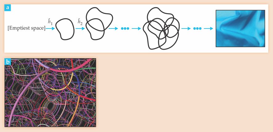
Rovelli and Smolin arrived at a picture of spatial atoms, not point-like or spherical but one-dimensional, extended along loops: Space is a giant molecule woven from threads, as schematically illustrated in figure 4. A single ladder operator raises the geometric excitation level—the atomic size of space—by a smallest, discrete, Planckian unit. One can eliminate excitations using inverse operators. Their destructive work reduces the size of space and eventually brings us back to ψ0, the state of unexcited, emptiest space.

Figure 4. Starting with emptiest space in its state ψ0, ladder operators ĥi in loop quantum gravity generate geometry. (a) As illustrated in this schematic, the geometry is atomic and polymer-like, with complicated meshes building space on small scales. Only on distances much larger than the mesh spacing does general relativity’s curved continuum emerge. (b) The spin network presented in this simulation is a more rigorous way to represent multiple applications of ladder operators. Different colors here represent different degrees of excitation.
In the cosmos, space grows dynamically, without the willful action of mathematicians applying ladder operators. To describe those dynamics, a theory needs to furnish a quantization of Einstein’s equation, some Schrödinger-equation analogue, but one that does not assume an absolute time. We are brought back to hypersurface deformations, which tell us how to change time and how spacetime evolves.
General relativity is complicated enough, so one cannot expect simple solutions for a quantum version. Even formulating potentially suitable evolution equations was difficult, but it is now possible thanks mainly to work by Thomas Thiemann 7 in 1996. What remains open is the question of whether the quantum theory is consistent and covariant—that is, whether it leads to a quantum version of hypersurface deformations that remains indifferent to specific coordinate choice.
The discrete nature of space affords several mathematical advantages but also includes dangers regarding physical consequences. Meddling with Lorentz symmetries should not be done lightly. 8 The radical deconstructivism inherent in a loopy ladder that allows one to descend all the way down to emptiest space and to climb back up harbors an immense creative power—but whether loop theorists can tap and control that force remains to be seen.
A hell of a state
A whole world rests on emptiest space, at least according to loop quantum gravity. Quantum physics of spacetime follows from the basic state ψ0 and the ladder operators. If that basic state is wrongly chosen, the whole theory must fall. It is important to characterize and understand ψ0, for it is unlike all ground or vacuum states physicists usually encounter. And not all characterizations may sound benevolent.
As a mathematical analogue of ψ0, Klaus Fredenhagen proposed a state of infinite temperature, in which all excitations are equally likely since there is no lack of energy. The unexcited state of quantum space resembles a matter state in which any energy excitation can be reached, a result (elaborated on in
Cosmologically, ψ0 is important because it satisfies all requirements for a Big Bang state that represents the universe at its densest moment: The temperature is infinite; there is no spatial extension in that emptiest space; and, based on a measure of entropy, ignorance is maximized. Ignorance may be a virtue when it comes to hell, but a lack of mathematical control over the State of Hell would seem to preclude physical predictions.
Given the extreme scales of quantum gravity, the only justifiable hope for probing the State of Hell must rely on obtaining indirect evidence, a situation not unlike that accompanying the 19th-century debates about the reality of material atoms. It was Einstein’s analysis of Brownian motion in 1905, and subsequent experiments by Jean Perrin, that convinced the majority. Despite the molecules’ tiny size, the sheer number of them colliding with suspended larger objects in a liquid causes visible motion. Observed and statistically analyzed, that motion provided quantitative evidence that was hard to reject even if atoms could not be seen directly. A half century later, impressive imaging techniques enabled atomic resolution, first achieved by Erwin Müller with field ion microscopy. But that accomplishment was not needed to establish atoms for real.
Quantum gravity faces similar problems, albeit on vastly different scales. Even to see indirect evidence, observers will need enormous magnification. Quantum-gravity researchers set their hopes on the largest microscope we have—the whole universe. By its very expansion, it magnifies everything. Many cosmic processes distort images, but with sophisticated techniques the images can still be compared against spacetime theories to decipher information about microscopic structures.
To some extent, the situation confronting loop-gravity theorists is similar to that faced by condensed-matter physicists—with spacetime atoms instead of material ones. As with matter, it is extremely difficult to do first-principles calculations that begin with a many-body Hamiltonian and arrive at quantum effects for macroscopic regions. Numerical simulations remain challenging but are now being developed for spacetime atoms thanks to work by Daniel Cartin, Gaurav Khanna, and others. Learning from condensed-matter physics, we gravity theorists need to develop good schemes for effective theories that offer approximate predictions for large-scale phenomena and that perhaps will help us to discover universal features insensitive to microscopic details. Unlike condensed-matter physics, however, quantum gravity cannot count on many experiments. Nevertheless, we are making progress, albeit slowly.
Deformed deformations
The structure of spacetime plays a foundational role for processes unfolding in it. One entry point for testing quantum gravity, therefore, is the form of hypersurface deformations. If we know how spacetime is modified by quantum effects, it may be possible to see some physics. It is not easy at all to modify the deformation algebra, just as it is difficult to meddle with Lorentz transformations; most attempts will simply destroy any symmetries. But if transformations can be preserved, albeit in a corrected form, they are good candidates for revealing universal phenomena.
Dimensional arguments suggest quantum effects would be of the order ρ/ρP, with ρ the average density. In all currently accessible regimes, that ratio is so tiny as to quench hopes for observational tests. However, theories of discrete spacetime have another option, thanks to a new scale: the discrete spacing L, or the average size of spatial atoms. Dividing by the Planck length yields a second dimensionless parameter, L/ℓP. The discrete spacing may well be different from ℓP, in which case the new parameter would be significant. We “only” need to evaluate our theory and see how L/ℓP enters into quantum corrections. That’s a difficult task because the existence of two dimensionless parameters ρ/ρP and L/ℓP precludes the use of dimensional arguments. But large-scale effects become possible, conceptually similar to Brownian motion that made the case for material atoms.
Loop quantum gravity gives rise to L/ℓP-dependent quantum effects called inverse-volume corrections. As shown in long, brave calculations by Mikhail Kagan and Golam Hossain, equation 1 gets modified to
T(N2)T(N1) − T(N1)T(N2) = S[α(N2∇N1 − N1∇N2)]. (2)
Evidently, quantum effects contribute to the commutator on the left-hand side of equation 2 a factor that is parameterized by α − 1, a result that has been confirmed by independent means, most recently by Adam Henderson, Alok Laddha, and Casey Tomlin.
For linear functions N as in figure 2, the relation between displacements and velocities, one of physics’s most elementary relationships, appears to be modified. According to the construction in figure 2, v is the velocity of a boosted observer who measures the motion of an object initially at rest. After a time Δt, one would expect the object to have moved a distance vΔt, but the result Δx = αvΔt is different—not much can be taken for granted if even space and time are quantum. The modified relation is not so surprising, though, if one thinks of spacetime as a condensed-matter analogue: Discrete matter structures often change propagation speeds compared with those in a structureless vacuum. In quantum spacetime, even the matterless vacuum has a structure that affects motion.
Propagation is important in cosmological theories of structure formation. When inhomogeneities are small, structure formation is described in terms of wave equations in an expanding cosmos. Normally, those waves propagate at the speed of light.
In quantum spacetime, electromagnetic and gravitational waves obey a wave equation with velocity √
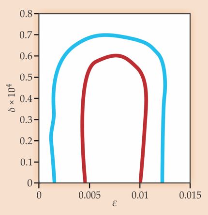
With additional observational data, particularly on cosmic gravitational waves, it may be possible to test loop quantum gravity along the lines indicated in figure 5. In any case, the theory does not make it easy to evade mounting observational pressure.

Figure 5. Observations of the cosmic microwave background and other data limit the size of the inverse-volume correction δ = α − 1 (see equation 2). This likelihood plot combines δ with a parameter ε that distinguishes between various possibilities for cosmic inflation. The lines bound regions in which δ and ε must lie with a likelihood of 68% (red curve) and 95% (blue curve). The upper bound here is about four orders away from a theoretical limit δ = 10−8 below which the discrete spacetime theory used to generate the curves is no longer consistent. As the cosmological data improve, the consistency of discrete spacetime theories will come under ever more rigorous observational scrutiny. (Figure by Shinji Tsujikawa, Tokyo University of Science; adapted from ref.
Back to the beginning
What happened deep within the high density of the Big Bang, a singular moment in general relativity? Was it the beginning of the universe or some transition phase? The simplest nonsingular scenarios are bounce models, which involve alternating epochs of collapse and expansion. 9 However, general relativity can realize such schemes only with rather contrived forms of matter. And in quantum gravity, high densities remain poorly controlled. Only partial, though fascinating, indications exist at present.
Loop quantum cosmology, 10 the application of loop quantum gravity to cosmology, eliminates the classical singularity; it describes the universe by a wavefunction that extends uniquely to times “before” the Big Bang. A well-knit plot has neither an accidental beginning nor an accidental end, according to Aristotle’s Poetics. Loops knit the spacetime story well, without the accident of a singularity.
“Before” here is in quotes because the notion of time in quantum spacetime may not agree with our intuitive temporal sense. Irrespective of what time means, however, its atomic nature implies that wavefunctions obey not differential equations but difference equations that discretely step over emptiest space. A valuable lesson: If we are discrete enough, we can avoid the State of Hell.
The equations of loop quantum cosmology specify what happened at and “before” the Big Bang, but many unknowns remain. Detailed information comes only from models that, like the quantum harmonic oscillator, can easily be solved but are too simple for general conclusions. Still, potential effects can be suggested, as shown by Leonardo Modesto, Jorge Pullin, Parampreet Singh, and others.
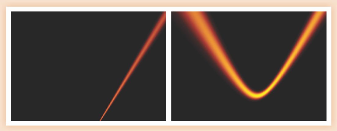
Bounces seem possible; figure 6 shows a sample calculation. But a bounce is a temporal scenario and requires good knowledge of the nature of time.

Figure 6. A simple quantum-cosmology model shows how the wavefunction for the volume of space changes as a function of time and replaces the classical Big Bang singularity (left) with a bounce (right). The bounce shown here, obtained analytically, had first been seen numerically
Out of time
At near-Planckian densities, hypersurface deformations are modified so dramatically that the quantum correction α is negative, as pointed out by Juan Reyes, Thomas Cailleteau, Jakub Mielczarek, Aurélien Barrau, and Julien Grain. Cosmological excitations are no longer subject to wave equations: Space and time derivatives enter with the same sign and appear in elliptic rather than hyperbolic partial differential equations.
For the special case of linear N, as in figure 2, α < 0 in equation 2 seems to say that an object forced to move with positive velocity experiences a negative displacement. Such intransigent behavior can more meaningfully be interpreted as a change of signature. When α turns negative, we no longer have spacetime. Instead, we have a quantum version of 4D space with no timelike direction.
A dense universe runs out of time. Bounces such as the one shown in figure 6 are not realized in a temporal sense. For the eras of collapse and expansion during which the universe is not so dense, α is positive and spacetime exists; the spacetimes of those epochs can be extended across the timeless Big Bang. But the collapse and expansion eras are not causally connected, and in particular, not all information can be transmitted between them. (How much can be conveyed is an active research question.) The transmutation from 4D space to spacetime, at a density for which α runs through zero, marks the beginning of our cosmic era: a meaningful moment, nonsingular and yet unprecedented.
Loop quantum gravity suggests that the universe does not begin with a big bang, nor does it follow cyclic behavior with causally connected periods of collapse and expansion. Instead, the theory offers a mixture of cyclic and monotonic worldviews, with a pre-history before the Big Bang but also forgetfulness that grants a clean slate afterwards. One can avoid dangerous entropy growth, a problem of cyclic models identified by Richard Tolman as early as the 1930s. Those features have been derived, not postulated. But before we can consider them reliable, the theory itself must be completed and empirically tested. We are not able to observe the high-density phase directly, but by delicate trickle-down effects in accessible background radiation, the theory, and by extension its strange consequences, can be falsified.
Box 1. Ladder operators
Ladder operators in loop quantum gravity have a classical correspondence in the magnetic flux computed from the vector potential A. The magnetic flux is the line integral of A along some loop ℓ with tangent tℓ. If we quantize the analogous gravity field Ai and take the exponential of the line integral, the result, called a holonomy ĥℓ, obeys the commutator relation [ P̂, ĥℓ] ∝ tℓĥℓ with a triad operator P̂, of the same form as is satisfied by the energy and ladder operators for the harmonic oscillator.
The harmonic oscillator has raising operators ↠that increase the energy via â†∣n〉 ∝ ∣n + 1〉 and lowering operators â that satisfy â∣n〉 ∝ ∣n − 1〉. Their role as ladder operators follows from commutators with the energy operator Ê: [Ê, â†] = Ê↠− â†Ê = ℏωâ†. If Ê∣n〉 = En∣n〉, Ê(â†∣n〉) = (â†Ê + [Ê, â†])∣n〉 = (En + ℏω)â†∣n〉.
In the same way, holonomies function as ladder operators that raise the excitation level of P̂ and change distance measurements.
Box 2. State of Hell
As described in
However, loopy ladder operators and the states they connect differ from the harmonic-oscillator ladders and states because the loopy ladder’s relation with the fields Âi and P̂i is different from the relation of the harmonic-oscillator ladders with position and momentum: For the harmonic oscillator, the ladders ↠and â are linear in position and momentum, not exponentiated operators as in the loopy case. To compare the models, one can compute expectation values of exp(iklx̂), obtained simply by replacing the gravitational  field in the flux integral with the position x̂. Then the ground-state expectation value for the harmonic oscillator would not vanish for k ≠ 0, but rather would yield a Gaussian function in k. No finitely excited state of the harmonic oscillator or of particle physics can produce the loop result. Quantum field theory, though, provides a state that can—the infinite-temperature state that inspired Klaus Fredenhagen to call ψ0 the State of Hell.
References
1. P. A. M. Dirac, Proc. R. Soc. London A 246, 333 (1958). https://doi.org/10.1098/rspa.1958.0142
2. S. A. Hojman, K. Kuchař, C. Teitelboim, Ann. Phys. (NY) 96, 88 (1976). https://doi.org/10.1016/0003-4916(76)90112-3
3. For an introduction, see, for example, R. Gambini, J. Pullin, A First Course in Loop Quantum Gravity, Oxford U. Press, New York (2011);
M. Bojowald, Once Before Time: A Whole Story of the Universe, Knopf, New York, (2010);
The Universe: A View from Classical and Quantum Gravity, Wiley-VCH, Weinheim, Germany (2013).4. See, for example, C. Kiefer, Quantum Gravity, Oxford U. Press, New York (2004);
D. Oriti, ed., Approaches to Quantum Gravity: Toward a New Understanding of Space, Time and Matter, Cambridge U. Press, New York (2009).5. C. Rovelli, L. Smolin, Nucl. Phys. B 331, 80 (1990). https://doi.org/10.1016/0550-3213(90)90019-A
6. A. Ashtekar, Phys. Rev. D 36, 1587 (1987). https://doi.org/10.1103/PhysRevD.36.1587
7. 7. T. Thiemann, Phys. Lett. B 380, 257 (1996); https://doi.org/10.1016/0370-2693(96)00532-1
T. Thiemann, Class. Quantum Grav. 15, 839 (1998). https://doi.org/10.1088/0264-9381/15/4/0118. J. Polchinski, Class. Quantum Grav. 29, 088001 (2012). https://doi.org/10.1088/0264-9381/29/8/088001
9. For a review, see M. Novello, S. E. Perez Bergliaffa, Phys. Rep. 463, 127 (2008). https://doi.org/10.1016/j.physrep.2008.04.006
10. M. Bojowald, Living Rev. Relativ. 11, 4 (2008); http://www.livingreviews.org/lrr-2008-4
Quantum Cosmology: A Fundamental Description of the Universe, Springer, New York (2011).11. M. Bojowald, G. Calcagni, S. Tsujikawa, Phys. Rev. Lett. 107, 211302 (2011). https://doi.org/10.1103/PhysRevLett.107.211302
12. A. Ashtekar, T. Pawlowski, P. Singh, Phys. Rev. Lett. 96, 141301 (2006). https://doi.org/10.1103/PhysRevLett.96.141301
More about the authors
Martin Bojowald is a professor of physics at the Pennsylvania State University in University Park.


