Auralization of spaces
DOI: 10.1063/1.3156831
In physics and other sciences, numerical simulation is an indispensable tool for describing and understanding complex phenomena. Examples abound, particularly in particle and wave propagation and the study of spatial and temporal evolution, such as of irradiation or pollution. Visualization is a familiar and useful companion tool in that respect, to illustrate multidimensional physical data such as electron shells, for example, or to graph distributions of geophysical stresses and strains. In those depictions and innumerable others, a physical quantity is expressed in a color scale. Often, large values are depicted by red and small values by blue, a scheme that mimics the subjective impression of heat. Physical or other data are thus transferred to an intuitive scale to match the needs of human visual perception.
Visualization is often used in the field of acoustics as well—for instance, to mark loud and quiet zones in noise maps with hot and cold colors. But let’s stop here and ask ourselves, Why are acoustic phenomena mapped so that they provide sensory input for the eye and not for the ear? Traditionally, the eye provides the main sensory input while we are reading. That process starts in primary school and continues through our university education. We listen to teachers and professors speak, but we focus on the meaning and rarely if ever on the sounds themselves. Mathematical, physical, chemical, and biological contents of learning are illustrated on printed matter by using diagrams or figures. Today, however, printed matter is complemented by electronic media, which can involve the eye and the ear equally and without restriction. In education, research, and consulting, discussions of acoustic phenomena are currently undergoing a revolution as the expression of sound in numbers and colors changes and an expression in “audible data” becomes possible. The process of making acoustic data audible is called auralization. The same concept can even be extended to include the auralization of data from nonacoustic phenomena, for which it is usually called sonification.
In auralizing spaces, one tries to simulate the effect that rooms have on sounds. Concert-hall acoustics serves as an example to understand the sound heard from a musical instrument. Without the room, the sound would be weak in intensity and poor in musical expression. The room is part of the musical experience: It adds strength and reverberation and makes the sound “spatial.” The difference between the so-called dry instrument sound and the sound in a room is the focus of architectural acoustics, a discipline founded some 100 years ago by Wallace Clement Sabine based on his studies of Boston’s Symphony Hall. 1 Today, architectural acoustics, its physics, and its hearing psychology are well understood in principle.
Room acoustic simulation in short
Wave physics in rooms can be described in the time domain or in the frequency domain. In the frequency domain, the ansatz of harmonic functions reduces the wave equation for the sound pressure p,
to the Helmholtz equation ▽2 p + k 2 p = 0. Here, c is the speed of sound, k the wave number (2π f/c), and f the frequency.
For a rectangular shoebox shape of dimensions L, W, and H, the boundary conditions are easy and the modes (room resonances) can be counted by natural numbers l, m, and n:
The Helmholtz equation can also be solved for any room shape and boundary condition by using numerical methods. The resulting modes are basically of the same quality as for the shoebox room.
Energy losses at the room boundaries give each mode a certain half-width in the sound-pressure frequency response. Because the density of modes increases with f2 , the acoustic behavior is characterized by two domains—one exhibiting modal behavior and one in which individual modes cannot be resolved and the behavior is statistical. As shown in this figure of sound-pressure magnitude |p| at an arbitrary point as a function of normalized frequency, the two domains are separated by the Schroeder frequency
where the reverberation time T is in seconds and the room volume V is in cubic meters.

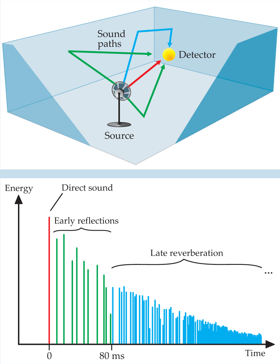
In another model of wave propagation in the room, one works in the time domain and considers the opposite of harmonic signals—the Dirac δ-function pulse and its propagation as a wavefront. As in geometrical optics, we can describe the wavefront by rays: Sound rays are emitted from the source, undergo specular reflections off smooth walls or Lambert scattering off irregularly shaped surfaces, and may reach a receiver (listener) after a finite travel time and energy loss. For the geometric model to be relevant, the surface dimensions must be large compared to the wavelength. Wave effects such as modes and diffraction are neglected. In the case of a specular reflection, the sound paths can also be constructed deterministically by using mirror-image sources, a method akin to that of mirror charges above a conducting surface. The plot of energy versus travel time is called the room impulse response (see figure

Figure 1. Room impulse response. (a) The sound source is modeled by omnidirectional ray emission. Four of the paths that reach the detector are shown. The paths reflect off the walls and arrive at different times and with different sound energies, which determine the positions and amplitudes of the corresponding peaks in the room impulse response. (b) In the total room impulse response, peaks are derived from numerous sound paths originating from all directions of emitted rays. The earliest peak is the direct sound. The early reflections that arrive within the next 80 ms determine the sound’s spatial impression.
The heart of the computer algorithms for ray tracing or mirror images is determining the points where ray vectors intersect infinite planes and testing whether those intersection points are in polygons that describe the portions of the infinite planes where the actual room boundaries (walls, floor, doors, windows, ceiling, reflector panels, and so forth) are located. The computational challenge is the time needed to consider all the permutations of boundary-to-boundary combinations. For large problems—room models with more than 1000 polygons—data structures such as beam trees can efficiently reduce computation time.
The
Basics and limits of room acoustics simulation
| Wave method | Ray-tracing method | |
|---|---|---|
| Basis | Modes, diffraction fields | Reflections, reverberation |
| Room size | Small, typically < 100 m3 | Large, typically > 100 m3 |
| Frequency range | Low, f ≪ fs , typically < 200 Hz | High, f ≫ fs , typically > 200 Hz |
| Sound signal | Pure tone, narrowband | Transient, broadband |
| Computational method | Numeric, analytic | Ray tracing, mirror images |
| Most important limitation | Computation time | Geometrical acoustics |
| Application | Control rooms for recording, music, and talk studios; vehicle cabins; rooms in dwellings; classrooms | Classrooms; theaters; concert and opera halls; churches; public spaces; workrooms; factories |
Basics and limits of room acoustics simulation
Basis |
Modes, diffraction fields |
Reflections, reverberation |
Room size |
Small, typically < 100 m3 |
Large, typically > 100 m3 |
Frequency range |
Low, f ≪ fs , typically < 200 Hz |
High, f ≫ fs , typically > 200 Hz |
Sound signal |
Pure tone, narrowband |
Transient, broadband |
Computational method |
Numeric, analytic |
Ray tracing, mirror images |
Most important limitation |
Computation time |
Geometrical acoustics |
Application |
Control rooms for recording, music, and talk studios; vehicle cabins; rooms in dwellings; classrooms |
Classrooms; theaters; concert and opera halls; churches; public spaces; workrooms; factories |
Architectural acoustics
Sound generally propagates from the source into free space and is distributed over a range of directions. In the far-field approximation, which holds quite well for distances larger than 2 m, the radiated sound pressure depends only on the direction and on the 1/r distance law of spherical wave propagation. In a room, the primary sound wave is diffracted and scattered by obstacles such as rows of chairs or columns and reflected from room boundaries. So to understand the effect of the room, one has to know the amount of diffraction, scattering, and absorption (or reflection).
The physics expressed in the linear theory of sound is rather similar to electromagnetic wave theory, and thus we find similar approximations of scattering, diffraction, and plane-wave reflection. The key to describing those wave effects is the Helmholtz number k·a, the product of the wavenumber k = 2π/λ, where λ is the wavelength, and the characteristic dimension a. However, consider that sound frequencies in the audio range from 20 Hz to 20 kHz and characteristic room and obstacle dimensions vary between 5 cm and 50 m. Thus the range of Helmholtz numbers covers six decades. Approximations such as Mie or Rayleigh scattering and Fresnel or Fraunhofer diffraction cannot be applied across the whole frequency range.
The numerous eigenfunctions (modes) in a bounded medium create further complications. We can identify in bounded spaces acoustic modes equivalent to the modes we can find in lasers, optical fibers, or waveguides, particularly if the geometry is easily defined by Cartesian, cylindrical, or spherical coordinates. The analytical solutions of the acoustic Helmholtz equation give excellent insight into the acoustic field in rooms (see
When studying sound-field physics by using the stationary solution to the Helmholtz equation, one expects the sound perceived in rooms to be an awful cacophony: It varies in space—the sound level of the various listening areas in concert halls will differ greatly—and it statistically fluctuates with random phases. Our experience of listening to sound in rooms, however, is completely different: Sound in rooms is quite acceptable, and “room effect,” or spatial sound, is even desirable and often added by using effect processors in music production. How is that possible?
In answer, please note that you were led down a wrong track when we discussed wave physics and the stationary case—the so-called “pure tone” or “acoustic laser.” The pure physical approach based on harmonic excitation obscures crucial points of listening in rooms. Consider two facts:
Real-world sound signals are usually not dominated by pure tones but by tone mixtures, noise, and transients.
Our listening experience in a room, compared with a free field (outdoors), is characterized by reverberation—a dynamic phenomenon in time.
Thus we need to extend the discussion on room acoustics from pure tones and sound pressure distributed in space toward a concept of sound propagation in time. Apart from specific problems such as low-frequency hums or feedback loops in public-address systems (examples where pure tones are relevant indeed), the time-domain approach gives much better insight into the psychoacoustic effects of sound in rooms.
The approach of acoustics in the time domain is best understood as a form of particle or ray tracing. We are now in the field of geometrical acoustics, the basis for simulations and auralizations of large spaces. In contrast to wave physics, the fundamentals are energy carriers such as particles that propagate at the speed of sound, hit room boundaries, and occasionally reach receivers (listeners). The room’s sound field is now composed of a series of reflections, each with a specific delay and energy (see
Imagine being a listener in a room and perceiving an impulse-like handclap sound from a source. The direct sound determines the localization of the source. It is the first acoustic information to reach you, and its arrival time depends on the distance between you and the source. The reflections arriving within 80 ms of the direct sound form a cluster of so-called early reflections that produce specific subjective effects—such as clarity, intimacy, and envelopment—on the overall impression of spatial room sound. 2–4 Reflections with delays longer than 80 ms form the reverberation in its specific, data sense. (Note the distinction between a reflection and an echo. In room acoustics, an echo is a strong reflection with a delay larger than, say, 100 ms that creates a perceived repetition of the sound.)
In a three-dimensional space, the probability of similar delays increases with time t, resulting in a reflection density that scales as t 2. The density of modes in frequency domain also increases as f 2. Such cross-domain analogies are fascinating. Manfred Schroeder pointed out the time–frequency correspondence in the transition from the modal regime to the statistical regime in wave fields. 5
The impulse response consists of parts that depend on the source and listener positions in the room and parts that are statistical in nature and similar throughout the space. Understanding the decomposition is essential: In simulations of room acoustics and in auralizations, one must balance the computational complexity of achieving physical correctness on the one hand and the speed and ease of application and the perceived realism on the other. Therefore, one typically uses mixed strategies that combine exact calculations of delay and energy with stochastic components that approximate the reverberation tail. 6 The quality of simulation programs, if applied correctly, is about the same as the quality of state-of-the-art acoustic measuring equipment. The uncertainties or deviations from the “true” result are of the order of magnitude of the so-called just-noticeable differences, the resolution scale of human acoustic perception.
Sound signal processing
Having methods available to calculate the impulse response, we can prepare the next step of the auralization. Through geometrical acoustics and stochastic methods such as ray tracing and radiosity—which simulates the diffuse propagation of sound—one can identify the energy, delay, and direction of incidence for the direct sound and each reflection. The key algorithm in audio signal processing is convolution.
In physics, convolution is commonly used to calculate joint probability density distributions in electron clouds or to extract spectral sensitivity functions of detectors from measurement data. In audio engineering, convolution is used to filter sound. Such filters may represent simply a coloration of sound (such as an equalizer) or any other linear operation on the time-dependent audio signals(t) (see

Figure 2. Auralizing rooms requires mapping the wave-propagation model to a signal-processing model. Reflections and other effects are represented by a binaural room impulse response h(t) that is calculated using ray tracing, image sources, and other computational techniques. The impulse response is convolved with the temporal function s(t) of a reverberation-free sound (such as a recorded source sound) to produce the spatial sound g(t) heard by the listener.
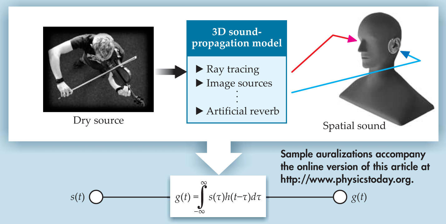
The sound propagation model in Figure
The HRIR is the inverse Fourier transform of the binaural head-related transfer function (figure

Figure 3. Sound goes binaural. Diffraction and reflection by the head and torso cause the sound field at the left and right ears to be different. Those effects are represented by head-related transfer functions. Filtering of monaural signals with HRTFs creates three-dimensional sound images. The transfer functions are usually defined in polar coordinates for the plane waves incident in a given direction. (a) A sample HRTF magnitude for the right (red) and left (blue) ears. (b) The corresponding, normalized head-related impulse responses, the inverse Fourier transform of the HRTFs. The HRIRs illustrate the amplitude and time difference of sound arriving at the ears. In this example, the sound is incident from the left side of the listener.
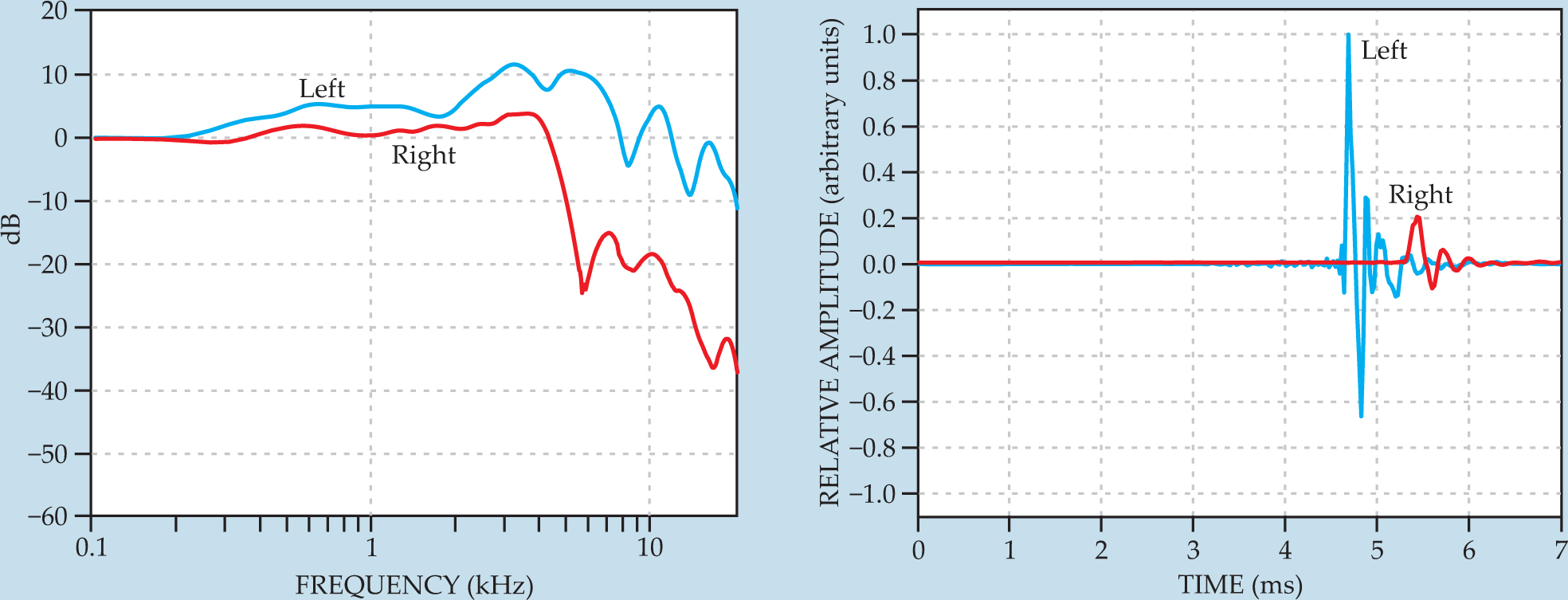
Binaural syntheses can be used for various acoustic scenarios in outdoor or indoor environments. Each sound path, including the direct sound and each reflection, must be filtered separately with the HRTF of the specific direction. The virtual acoustic signal at the listener is therefore consistent with the real sound field, including delayed repetitions of the original sound, and thus the impression of sound in the virtual space is auralized.
Auralization signal processing
Any sound signal s(t) can be decomposed into a series of weighted and delayed Dirac pulses δ(t) by using the convolution integral
The convolution partner of the signal can also be an impulse response function h(t) consisting of a series of impulses with different heights and delays:
One example of such a generalized impulse response function is the room response (see figure
In linear signal and system theory, the convolution with an excitation signal can be written as
The right-hand side can be straightforwardly interpreted: The signal g(t), which could be the sound signal heard by a listener, contains repeated versions of s(t) at each occurrence of a reflection path with retardation t i .
The task of room acoustic computer programs is to determine the history of rays or particles in those reflection paths that reach the listener. The needed data are the list of surfaces hit, their contribution to absorption and scattering, and the directions with respect to both source and listener. Including all relevant aspects of sound propagation, the contribution of a single reflection path to the impulse response is
The components in the above equation are the source directivity Γ, in source-related coordinates θ and φ; the spherical-wave spreading factor 1/cti ; the retardation ti ; the effective impulse response h surfaces of the boundaries involved (h surfaces can be calculated as the inverse Fourier transform of the product of the complex reflection factors at each boundary); and the binaural head-related impulse responses, HRIRr,l, in head-related coordinates ϑ and φ . Finally, the binaural impulse response, representing the signals at the left and right ears, is given by
The mathematical procedure of convolution can alternatively be expressed in the frequency domain by simple multiplication. The Fourier transform or its fast digital version, the FFT, is used to swap between time-domain and frequency-domain processing. For real-time processing, operations in frequency domain are typically faster, despite the computational load of the FFT.
Acoustic virtual reality
The auralized sound can be presented with an appropriate sound-reproduction system consisting of headphones, loudspeaker groups, or loudspeaker arrays. In each case, specific signal processing is used to implement the binaurally auralized spatial sound that will reach the listener’s ears. The quality of the systems used in acoustics research is superior to that of commercial surround-sound systems used in home theaters. Although similar to consumer electronics, the research systems provide exact sound localization in 3D space rather than a rough spatial effect of “left, right, or behind.” Accordingly, the listening room must be considered, too, because by its own reflections it will modify the sound field at the listener’s ears. An anechoic—that is, reflection-free—environment is therefore advantageous, except when using headphone reproduction. Headphones, though, require exact equalization and adaptation to individuals.
The problems of the sound reproduction may be reasonably resolved, so the last frontier to be tackled is real-time auralization. A real-time performance is one of the three elements of virtual reality (VR). The other two are multimodality (addressing not only visual senses but also auditory, tactile, and other senses) and interactivity (allowing the user to move within the virtual environment, change objects, and the like). With a 3D representation of the virtual environment, the user will experience immersion, one characteristic feature of VR systems.
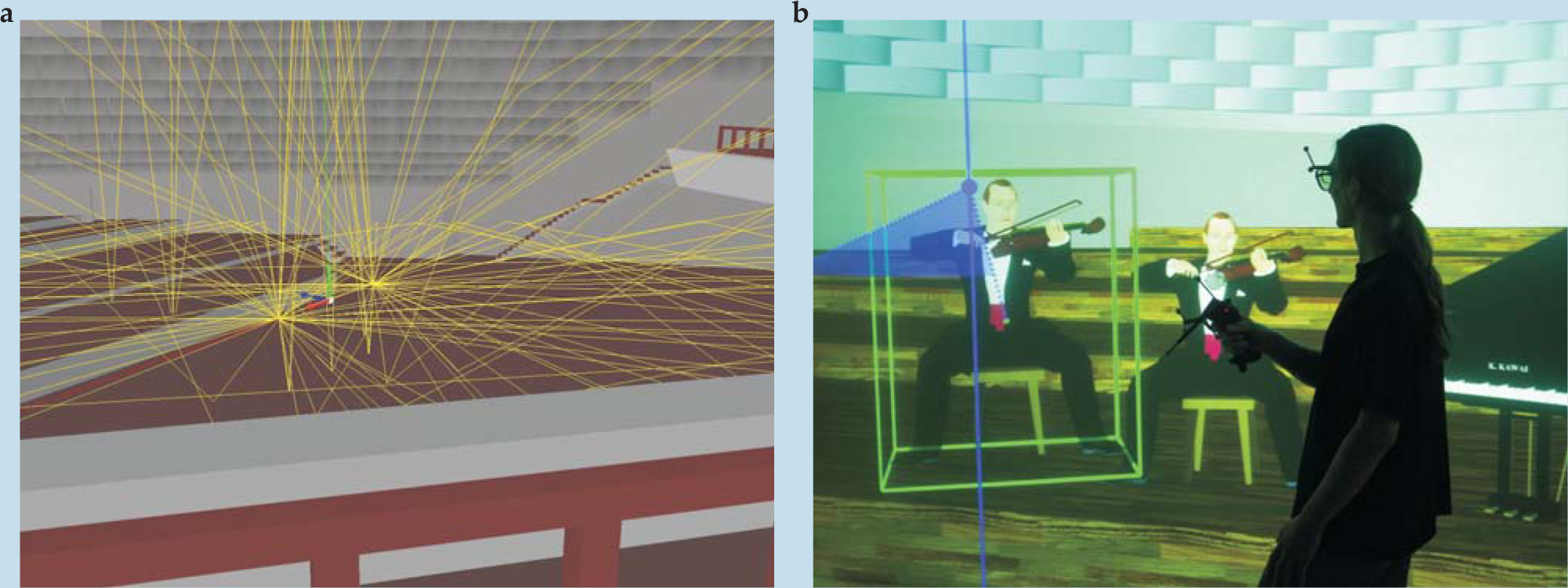
Everything described so far about auralization also applies to VR settings: simulation of sound-field physics, signal processing for auralization, and 3D sound reproduction. But if the system is supposed to be dynamic, the position of the user must be measured (using head-tracking techniques) and transferred to an adaptive process (see figure

Figure 4. Virtual room acoustics. Integration of virtual reality and acoustics in a virtual concert hall. (a) The paths in yellow are calculated to be audible for a certain virtual listening position. (b) In an interactive virtual reality, such as this CAVE-like environment, the auralization needs to be updated every time the listener’s position or head orientation changes. The Cave Automatic Virtual Environment was first presented by Carolina Cruz-Neira and colleagues at the University of Illinois.
Room acoustic simulation remains an active area of research. From the above introduction to sound-field physics, it becomes clear that the particle or ray approach implemented in room acoustic simulation is only an approximation at higher frequencies. For small rooms or low frequencies, low-frequency modes will be significant. Few methods can calculate wave and particle acoustics simultaneously and thus cover the whole range of audible frequencies. Diffraction is hardly accounted for in a satisfactory way as yet. Efforts to extend uniform geometrical diffraction theory 8 and other geometrical diffraction models to include multiple combinations of diffraction and reflection are promising. 9 More applications are also being designed and tested.
Auralization is an important tool for test scenarios not only in room acoustic VR research, 10–12 but also in areas such as psychology (orientation, attention, behavior), human hearing, and neural processing, to name only a few. Obvious applications of auralization are teleconferencing, entertainment systems, and computer games. Even without those uses, simulations and auralizations will make progress on their own, if Moore’s law of exponential increase in computer power remains valid for some years. But auralization is not merely a function of computer speed and memory size: Sound-field physics is more complex than accounted for in geometrical acoustics today, and better modeling of sound-field physics is needed. The goal of auralization is to create an auditory event that sounds correct: Psychoacoustic effects determine the precision to which the sound field needs to be understood and re-created. Determining the balance between physical accuracy and audible effects remains an interesting and challenging interdisciplinary problem.
References
1. W. C. Sabine, Collected Papers on Acoustics, Harvard U. Press, Cambridge, MA (1922), reprinted by Dover, New York (1964).
2. H. Kuttruff, Room Acoustics, 5th ed., Taylor and Francis, New York (2009).
3. L. L. Beranek, Concert Halls and Opera Houses: Music, Acoustics, and Architecture, Springer, New York (2004).https://doi.org/10.1007/978-0-387-21636-2
4. M. Barron, Auditorium Acoustics and Architectural Design, Spon Press, New York (1993).
5. M. R. Schroeder, J. Acoust. Soc. Am. 99, 3240 (1996). https://doi.org/10.1121/1.414868
6. M. Vorländer, Auralization: Fundamentals of Acoustics, Modelling, Simulation, Algorithms and Acoustic Virtual Reality, Springer, Berlin (2008).
7. J. Blauert, Spatial Hearing: The Psychophysics of Human Sound Localization, MIT Press, Cambridge, MA (1996).
8. M. A. Biot, I. Tolstoy, J. Acoust. Soc. Am. 29, 381 (1957). https://doi.org/10.1121/1.1908899
9. U. P. Svensson, R. I. Fred, J. Vanderkooy, J. Acoust. Soc. Am. 106, 2331 (1999). https://doi.org/10.1121/1.428071
10. T. Lokki, L. Savioja, R. Väänänen, J. Huopaniemi, T. Takala, IEEE Comput. Graphics Appl. 22(4), 49 (2002). https://doi.org/10.1109/MCG.2002.1016698
11. T. Funkhouser, N. Tsingos, I. Carlbom, G. Elko, M. Sondhi, J. E. West, G. Pingali, P. Min, A. Ngan, J. Acoust. Soc. Am. 115, 739 (2004). https://doi.org/10.1121/1.1641020
12. T. Lentz, D. Schröder, M. Vorländer, I. Assenmacher, EURASIP J. Adv. Signal Process. 2007, 70540 (2007).https://doi.org/10.1155/2007/70540
13. C. Cruz-Neira, D. J. Sandin, T. A. DeFanti, Proceedings of the 20th Annual Conference on Computer Graphics and Interactive Techniques, Association for Computing Machinery, New York (1993), p. 135.https://doi.org/10.1145/166117.166134
More about the authors
Michael Vorländer directs the Institute of Technical Acoustics at RWTH Aachen University in Aachen, Germany.
Michael Vorländer, RWTH Aachen University, Aachen, Germany .


