Atomic clocks for controlling light fields

Norman Ramsey, who died in November 2011 at age 96, revolutionized the measurement of time by inventing, in 1949, the separated-fields atomic interferometer. His immediate (and inspired) quest was to improve the spectral resolution of magnetic resonance using molecular beams. For that story, see Daniel Kleppner’s account on page 25 and Ramsey’s own description of the achievement on page 36 . But Ramsey’s device finds its most widespread application in atomic clocks, which count the oscillations of atomic transitions with extraordinary precision. ^{1 , 2}

Ramsey proposed the hydrogen maser about a decade after his invention, shortly after Kleppner joined his group, and together they demonstrated one in 1960. Atomic-beam clocks and hydrogen masers now underlie the operation of the modern global positioning system. But the GPS is but one of the many uses of atomic clocks.

In fundamental physics, atomic clocks and their ability to time electromagnetic signals are used to test special and general relativity. They are also fantastic tools to probe quantum theory in experiments that send a stream of atoms through photons trapped in cavities. ³ In the context of probing quantum theory, a central goal is not to time light but rather to tame it. Thanks to progress in quantum optics made since the 1980s, such cavity quantum electrodynamics experiments can produce fields with unusual or tailor-made properties (see Physics Today, December 2012, page 16 ). The fields may thus be used to explore quantum information processing and to deepen our basic understanding of atom–photon interactions. Both projects exploit the control and flexibility that cavity quantum electrodynamics provides.

Ramsey interferometers as clocks

Suppose you want to determine the rotation frequency ν₀ of a wheel. Stroboscopic illumination with light pulsed at nearby frequency ν makes the wheel appear to revolve slowly at a frequency equal to the difference ν₀ − ν. So one can deduce ν₀ by simply observing at time t the apparent phase 2π(ν₀ − ν)t of a spoke. Counting the oscillations of atomic electrons is more challenging. The method for doing so, however, is similar and relies ultimately on a stroboscopic measurement performed using the Ramsey interferometer, illustrated in figure 1a.

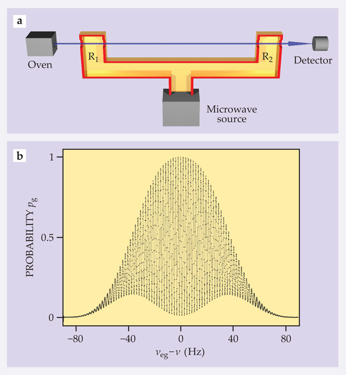
To appreciate how the device works, imagine a beam of atoms effusing from an oven across two sections, R₁ and R₂, of a waveguide fed by a microwave source whose frequency ν is nearly resonant with that of the transition ν_eg between an initial atomic ground state g and an excited state e. As they successively cross those sections, the atoms are irradiated by two microwave pulses separated by a time interval Δt. In each pulse the resonant field periodically shuffles them between ground and excited states, a reversible process known as Rabi oscillation. The R₁ pulse, set to a quarter period of the oscillation, places the atoms in a coherent and equally weighted superposition of e and g.

That superposition freely evolves at frequency ν_eg as the atoms travel from R₁ to R₂. Meanwhile, the field evolves at ν. The atomic superposition and field thus accumulate a phase difference Δφ = 2π(ν_eg − ν)Δt. If Δφ = 2kπ, where k is an integer, the R₁ and R₂ pulses are in phase with the atomic coherence and their effects add constructively: The atoms undergo a half-period Rabi oscillation and end up in e. If Δφ = (2k + 1)π, the second pulse undoes the action of the first and leaves the atoms in g.

In general, atoms end up in their ground states or excited states with probabilities p_g = 1 − p_e = (1 − cosΔφ)/2, which can be measured by accumulating statistics provided by a state-resolving detector outside the waveguide. As ν is swept through ν_eg, the probabilities p_g and p_e exhibit interference fringes whose spacing scales as 1/Δt.

Locking the microwave frequency on the central fringe at ν = ν_eg thus produces a time standard locked to the regular ticking of the atomic electrons. For narrow fringes, Δt should be large. Atomic fountain clocks therefore interrogate slow atoms,⁴ whose velocity has been reduced by laser cooling to around 10 cm/s. As shown in figure 1b, an interrogation time Δt around 1 s results in a fringe spacing of about a hertz.

Averaging signals over a day achieves a frequency stabilization better than 10⁻⁷ of that spacing. The resulting clock uncertainty is 10⁻¹⁵, roughly 1 second in 30 million years. The microwave clock’s low frequency (9.2 GHz for the cesium hyperfine transition) is the limiting factor. A 100-fold smaller uncertainty, on the scale of a few seconds over the age of the universe, has recently been achieved using optical clocks. They count the much higher (1000 THz) frequencies of laser fields locked to the few-hertz-wide optical resonance of a single trapped ion. ⁵ The optical-frequency clocks, though, rely not on the Ramsey interferometer but on another amazing spectroscopic tool, the optical frequency comb ⁶ —a story for another time (see Physics Today, December 2005, page 19 ).

Detecting single photons

Ramsey clocks must be protected against stray electric fields and other perturbations that alter, even slightly, the atomic-state superposition. Although ingenious procedures can minimize the fields’ effects, it’s possible to turn that potential obstacle into an advantage. That has been our perspective for the past several years, working at École Normale Supérieure in Paris: We exploit the Ramsey interferometer’s extreme sensitivity to radiation as a tool for counting and manipulating photons without destroying them. ⁷

Pulling that off requires placing a photon-trapping cavity between the interferometer’s two microwave sections, as illustrated in figure 2a. As before, atoms interact with a microwave field in regions R₁ and R₂, but they now also pass midway between two highly reflecting mirrors. Crucially, the resonance frequency ν_C of that mirrored cavity is tuned away from ν_eg to prevent the atoms and the cavity from exchanging photons. Nonetheless, if any photons reside in the cavity, they do interact with the atoms, and those interactions shift the atomic transition frequency. That “light shift”—akin to the mutual frequency change experienced by two coupled nonresonant classical oscillators—is inversely proportional to δ = ν_eg − ν_C and directly proportional to the photon number n. As a result, the phase difference Δφ between the atomic coherence created in R₁ and the microwave pulse in R₂ is shifted by an additional amount nΔφ₀, where Δφ₀ is the phase shift per photon.

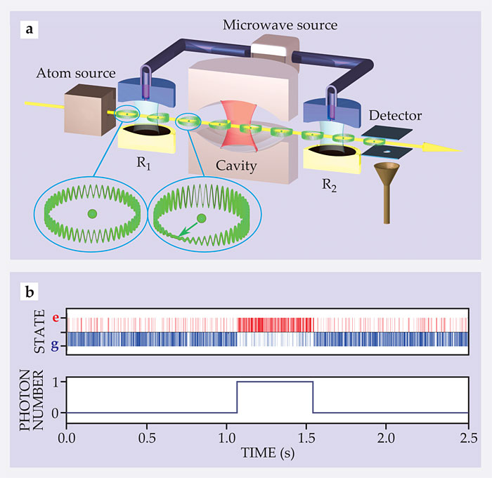
Single-photon sensitivity is reached using circular Rydberg states. They are prepared by exciting the valence electron of rubidium atoms into a circular orbit whose radius, in the micrometer range, is more than three orders of magnitude larger than that of rubidium’s ground state. Such a huge atom is a large antenna, extremely sensitive to nearly resonant fields. The electron wavefunction forms a circular traveling wave with an integer number—the principal quantum number—of de Broglie wavelengths along the orbit circumference.

The levels g and e correspond to principal quantum numbers 50 and 51, with e having a larger orbit and accommodating just one more de Broglie wavelength than g. A beam of atoms separated by a few centimeters passes through the interferometer at about 250 m/s. The first microwave pulse prepares a superposition of e and g; the two de Broglie waves interfere constructively on one side of the orbit and destructively on the other. With the electron density being crescent shaped, the atom acquires an enormous electric dipole that, like the hand of a clock, rotates at ν_eg = 51 GHz. After passing through the second pulse, the atoms enter a detector whose electric field ionizes them and can discriminate between e and g states.

Information about the photon number must be acquired before the field is lost through unavoidable leaking from the cavity. Mirrors of exceptionally high reflectivity are required. Made of copper coated with a thin layer of superconducting niobium, they are cooled to 0.8 K. They hold photons for a mean lifetime T_c of about 130 ms. During that time, light quanta bounce more than a billion times between the mirrors while hundreds of atoms traverse the trapping cavity.

At 0.8 K, according to Planck’s blackbody radiation law, the cavity is most often in its vacuum (n = 0) state, but a single photon is present 5% of the time. To observe that fleeting light quantum, we set Δφ₀ to π by adjusting δ. The Ramsey signal p_e is set at a fringe minimum so that when n = 0, the atoms are detected in g; its shift to a fringe maximum when n = 1 results in the atoms being detected in e. The sudden shift in the field intensity—a manifestation of quantum jumps between states—switches the detected atomic state and reveals the birth and death of a single photon (see Physics Today, June 2007, page 21 ).

Raw atomic detections, illustrated in figure 2b, are noisy because the correspondence between the presence of a photon and an atom’s state is inexact. Even so, one can discern after 1 s a clear upward quantum jump, indicating a photon in the cavity. That photon survived for another 0.5 s, roughly 4T_c. The longevity isn’t too surprising: As in any spontaneous decay, particles can, on rare occasions, outlive their natural lifetime by a large amount.

The same photon is “observed” by hundreds of nonresonant atoms, which are unable to absorb it; the detection is thus termed quantum nondemolition (QND). Whereas usual light detection annihilates a photon, a photon detected by QND remains in the cavity, ready to be detected again. Counting by this process prepares a quantum state with a well-defined photon number, known as a Fock state, which in this case is either the vacuum state ∣0〉 or one-photon state ∣1〉.

Counting multiple photons

For more variety, one can also count larger photon numbers. ⁸ To prepare a large field, one need only irradiate the central cavity with resonant microwaves. A small fraction of the photons scatter from the mirrors’ edges, become trapped in the cavity, and survive for a time T_c after the microwave source is turned off.

That operation places the field in a coherent state, the quantum state closest to the classical picture of an oscillating electric field with a well-defined complex amplitude. A classical field can be represented as a point in the phase plane, whose polar coordinates are the amplitude’s modulus and phase. The plane’s Cartesian coordinates x and p are the position and momentum of the field mode viewed as a one-dimensional harmonic oscillator.

Heisenberg uncertainty relations preclude perfect localization of the complex amplitude. Coherent states thus have a fuzzy phase and photon number. They are a quantum superposition of Fock states ∣n〉, the states containing exactly n photons. The photon number probability distribution is a Poissonian, with width √〈n〉 for average photon number 〈n〉.

The so-called Wigner function W provides a pictorial representation of the coherent state in the phase plane. The function is a quasi-probability distribution for the field amplitude. In loose terms, W is a wavefunction for the field amplitude and thus a fingerprint of the quantum state; more precisely, it’s a unique graphical representation of the density matrix, given by information on the field state from atoms that probe it in a QND way. ⁹ Figure 3a illustrates that for a coherent field with 〈n〉 = 2.5, the Wigner function is a Gaussian peak centered in phase space on the classical amplitude of the field.

How can we generalize the QND procedure to count the number of photons in a coherent state? Because a Rydberg atom sent through the cavity behaves like a clock whose rate is affected by each of possibly several photons in the cavity, the simplest procedure is to set the phase shift per photon to Δφ₀ = π/(n_m + 1), where n_m is the maximum likely number of cavity photons in the coherent state. There are then n_m + 1 values of p_e = 1 − p_g between 0 and 1. Those distinct probabilities are associated with n between 0 and n_m; determining p_e thus measures the photon number.

One atom, of course, is not enough to resolve the signal. It takes dozens of atomic detections to reduce the statistical noise in the determination of p_e below the roughly 1/n_m difference between p_e values for different photon numbers.

The actual procedure is a bit more involved. Instead of determining p_e, we perform a statistical analysis based on Bayes’s law of conditional probabilities. (See the Quick Study by Glen Cowan in Physics Today, April 2007, page 82 .) That is, we deduce from the successive detections of atoms that stream through the system an evolving photon number distribution. The distribution develops a peak on a single photon number after we’ve detected some 80 atoms over a span of 20 ms.

The information acquisition process using successive atoms captures the progressive collapse of the field’s wavefunction. The field starts as a coherent state without a well-defined number of photons, and it ends in a Fock state. The final photon number may thus be different from the initial average one. That difference arises not from an atom–field energy exchange but rather from the chance encounters the system makes as it evolves. Quantum mechanics predicts only probabilities, which are given by the photon number distribution in the initial state.

Figure 3b illustrates one realization of the experiment. At its start little information is available, so the initially inferred photon distribution is flat, between 0 and 7 possible photons. During the initial 20 ms the number evolves from an inferred average of 3.5 and quickly collapses to 5 photons. During its plateau at that number, we detect enough atoms streaming through the cavity to perform two independent measurements of n; both yield the same result and vindicate the QND nature of the process. As photons leak out from the cavity, one by one, subsequent measurements reveal a series of quantum jumps that lead inexorably to the vacuum state. Between jumps, the system converges to a new Fock state.

Figure 3c presents the measured Wigner function of the three-photon Fock state. ⁹ Its energy is well defined, but the phase isn’t, because W is rotationally invariant. Moreover, because the function takes both negative and positive values, the state defies description as a classically fluctuating amplitude given by a probability density. Fock states belong to the quantum realm and are fragile, all the more at high photon numbers: A statistical analysis of the jumps ¹⁰ reveals that the average lifetime of ∣n〉 is T_c/n.

Using atoms to juggle photons

The Ramsey interferometer’s utility goes well beyond counting. Its QND atomic-state measurements can be fed as input to a computer that then estimates the field state and decides how to react in order to bring the field to a desired state and keep it there. That feedback strategy tames the quantum field by preparing and maintaining a fragile Fock state for an indefinite time. ^{11 , 12} The method is analogous to juggling. The juggler looks at the balls he wants to keep on an ideal trajectory. His eyes are the sensors and the visual information is processed by his brain to determine the correcting actions of his hands, the actuators.

A quantum juggler, though, faces a challenge absent in the classical game. The mere action of observing photons has an unavoidable and unpredictable influence on them—the so-called back action. However, once an atom has been detected, the back action on the photon number distribution can be inferred using Bayes’s law. The computer can thus update the field state using the results of successive measurements. At each step, it evaluates a distance between the actual and target states and computes a response that minimizes the distance. As in classical feedback, the procedure is implemented in detection–correction loops until the target is reached. The computer then watches for quantum jumps and corrects for their effect.

What serves as the “hand” in this juggling game? In one version of the experiment, it is a classical light source—periodically injecting small microwave fields that, depending on their phase, increase or decrease the field amplitude. ¹¹ In a conceptually simpler version, ¹² the actuator is realized by atoms tuned in resonance with the cavity. They emit a photon if they enter the cavity in e and absorb one if they enter in g. The feedback process illustrated in figure 4, with an n = 4 Fock state as target, involves repeatedly sending a sample of a few nonresonant sensor atoms followed by a few resonant actuators.

Schrödinger cats and decoherence

Other nontrivial field states can also be prepared. Of particular interest is a Schrödinger cat state with a superposition of coherent states that have the same mean photon number and nearly opposite phases. ⁹ The preparation of such states illustrates an essential aspect of quantum physics—the complementary role played by energy and phase. As the Ramsey interferometer progressively pins down the photon number, and thus the field energy, it randomizes the field phase. The first Rydberg atom in the QND photon-counting procedure initiates that phase blurring. The e and g components of its state superposition shift the field phase in opposite directions by ±Δφ₀/2. Thus, after their interaction, the atom and the field are entangled in a global superposition of states. If Δφ₀ = π, the two components of the “atom + field” system are associated with two coherent states of opposite phase. The system is reminiscent of Schrödinger’s cat, suspended between life and death by its entanglement with a two-level atom.

Measuring the state of the atom as it leaves the cavity would reveal the field phase, project it into one of the two components of the superposition, and thereby lift the quantum ambiguity. The second Ramsey pulse is essential to maintain the ambiguity. It mixes e and g so that the final atomic detection does not yield information about the state of the atom in the cavity. As a result, the atom’s final detection projects the field into a superposition of the two coherent states.

Figure 5a presents the Wigner function of a Schrödinger cat state with 〈n〉 = 3.5. The two peaks correspond to the coherent components of the field, and the interfering pattern between them reflects the coherence of the superposition. ⁹ Fragile and ephemeral, Schrödinger cat states are ideal guinea pigs for exploring the decoherence by which quantum superpositions evolve into classical statistical mixtures. As photons are lost, the interference pattern of the cat state disappears within a time of T_c/〈n〉. Snapshots of the Wigner function during that time—figures 5b and c—show the evolution. (For a description of a preliminary version of the experiment, see Physics Today, July 1998, page 36 .)

The lifetimes of a Schrödinger cat and a Fock state are of the same order of magnitude for the same 〈n〉. The greater their energies, the greater the challenge to prepare such nonclassical states before they decay. The trend explains why it is difficult to prepare and observe pure quantum superposition states of macroscopic objects.

Building blocks

Ramsey conceived his interferometer as a tool for precision spectroscopy. As often happens with groundbreaking inventions, the tool has proven successful beyond the dreams of its designer. Not only can the interferometer measure time with fantastic accuracy, but, as we’ve seen, it provides an experimental format for manipulating quantum states. One motivation behind juggling light fields with atoms is that the tailor-made states one can produce are the building blocks for new ways of handling information. Quantum computing, for instance, explores methods for processing complex entangled states of information coded within two-level qubits. ¹³

In many schemes, such qubits are coupled via their interaction with quantum oscillators, which may consist of fields in cavities or mechanical oscillators such as vibrating atoms or ions in traps. ¹⁴ In one fascinating new development, qubits take the form of superconducting Josephson-junction circuits that behave as artificial atoms. ¹⁵ Compared to real atoms, the mesoscopic circuits are huge and therefore even more strongly coupled to RF resonators, which behave like our cavities (see Physics Today, July 2009, page 14 ). ^{16 , 17}

In each of those contexts—from trapped photons to vibrating ions and circuit resonators—the tricks of Ramsey interferometry can be applied successfully. Already they’ve been used to build quantum gates that couple qubits, to demonstrate quantum-computation algorithms, and to create nonclassical oscillator states and protect them against decoherence. Systems with greater complexity and sophistication are bound to follow.

References

1. N. Ramsey, Molecular beams, Oxford U. Press, New York (1985).
2. F. G. Major, The Quantum Beat: Principles and Applications of Atomic Clocks, 2nd ed., Springer, New York (2010).
3. S. Haroche, J.-M. Raimond, Exploring the Quantum, Atoms, Cavities, and Photons, Oxford U. Press, New York (2006).
4. P. Lemonde et al., in Frequency, Measurement and Control: Advanced Techniques and Future Trends, A. Luiten, ed., Springer, New York (2001), p. 131.
5. C .W. Chou et al., Science 329, 1630 (2010). https://doi.org/10.1126/science.1192720
6. T. W. Hänsch, Rev. Mod. Phys. 78, 1297 (2006). https://doi.org/10.1103/RevModPhys.78.1297
7. S. Gleyzes et al., Nature 446, 297 (2007). https://doi.org/10.1038/nature05589
8. C. Guerlin et al., Nature 448, 889 (2007). https://doi.org/10.1038/nature06057
9. S. Deléglise et al., Nature 455, 510 (2008). https://doi.org/10.1038/nature07288
10. M. Brune et al., Phys. Rev. Lett. 101, 240402 (2008). https://doi.org/10.1103/PhysRevLett.101.240402
11. C. Sayrin et al., Nature 477, 73 (2011). https://doi.org/10.1038/nature10376
12. X. Zhou et al., Phys. Rev. Lett. 108, 243602 (2012). https://doi.org/10.1103/PhysRevLett.108.243602
13. M. Nielsen, I. Chuang, Quantum Computation and Quantum Information, Cambridge U. Press, New York (2000).
14. D. Leibfried et al., Rev. Mod. Phys. 75, 281 (2003). https://doi.org/10.1103/RevModPhys.75.281
15. R. Schoelkopf, S. Girvin, Nature 451, 664 (2008). https://doi.org/10.1038/451664a
16. M. Hofheinz et al., Nature 459, 546 (2009). https://doi.org/10.1038/nature08005
17. B. R. Johnson et al., Nature Phys. 6, 663 (2010). https://doi.org/10.1038/nphys1710
More about the authors
Serge Haroche directs the Collège de France in Paris and is a researcher at École Normale Supérieure. Michel Brune (CNRS) and Jean-Michel Raimond (Pierre and Marie Curie University) both work at ENS.