Asteroseismology
DOI: 10.1063/PT.3.2783

At birth, most stars in our current galaxy look chemically the same: They are roughly 71% hydrogen, 27% helium, and some 2% heavier elements collectively labeled metals. Deep within their interiors, the pressure, density, and temperature are sufficiently high to achieve nuclear fusion of hydrogen into helium. For most of a star’s life, that and subsequent fusion reactions will generate the internal pressure force needed to counterbalance gravity and keep the star from collapsing on itself.
How brightly and how long a star burns, however, can vary greatly depending on its birth mass. Stars similar to the Sun, say, with a mass less than or equal to twice the solar mass M⊙, live billions of years but undergo only two nuclear cycles—hydrogen burning and helium burning—before dying quietly as carbon- and oxygen-rich white dwarfs.
At the other extreme, stars with mass greater than 8 M⊙ live just millions of years but manage to loop through many nuclear burning cycles. They eventually form an iron core, at which point their fate is a core collapse followed by a supernova explosion that leaves a neutron star or black hole as a remnant. Because the explosion delivers heavy metallic elements to the surroundings, the massive stars, despite being rare, are essentially the steel factories of the universe. Most of the carbon available today was produced by stars with masses between 2 M⊙ and 8 M⊙, which are much more abundant than the most massive stars. (For a more detailed discussion of stellar evolution, see reference .)
Although the broad characteristics of stellar evolution are well known, many of the details are murky. The standard way to probe stars’ evolution is to catalog their mean surface properties—namely, the total emitted energy, or luminosity L, and the effective temperature Teff, the temperature of a blackbody of equivalent luminosity. The two quantities are related to each other by the stellar radius R: L = 4πσR2Teff, where σ is the Stefan–Boltzmann constant.
Because a star’s evolution is appreciably affected by physical processes in its interior, however, measurements of surface properties leave many important questions unanswered. For instance, how do stars rotate internally as they age? How do their nucleosynthesis products mix? Do stars have an internal magnetic field? Understanding how interior processes influence a star’s birth, life, and death is essential to understanding the evolution of exoplanets, galaxies, and the universe as a whole.
Asteroseismology—the study of radial and nonradial stellar oscillations, or starquakes—has emerged as a promising tool with which to investigate the physical processes inside stars. By relating periodic fluctuations in a star’s brightness to the acoustic and gravity waves that cause them, asteroseismology offers tantalizing glimpses into stellar interiors. Able to reveal rich information about a star’s internal density, composition, rotation, and convective mixing, it is already beginning to challenge some long-held theoretical notions. As more stars are observed for the purposes of asteroseismic analysis, the technique could conceivably test and improve our knowledge of every juncture in a star’s life—from the moments just before it’s born to the time of its silent or fiery death.
Scratching the surface
As a star evolves, its luminosity and effective temperature change. The star’s evolution can therefore be charted as a path on a so-called Hertzsprung–Russell diagram (HRD), as shown in figure 1. Note that the luminosity of the various types of stars spans nine orders of magnitude, whereas the effective temperature spans less than two.

Figure 1. This Hertzsprung–Russell diagram shows the effective temperatures and luminosities of the various classes of seismically oscillating stars. At birth, all of the stars burn hydrogen in their core and lie on the red line, known as the main-sequence curve. After the core-hydrogen-burning phase, stars evolve off the main-sequence curve as they progress through a series of nuclear fusion cycles. (Solid black lines denote the predicted evolution for stars of various birth masses, with masses given in terms of the solar mass M⊙.) The Sun’s predicted path, including its denouement—shrinking into a cool, dense white dwarf—is indicated in green. The blue and orange shading corresponds to effective temperature. The hatching indicates the nature of the dominant oscillation modes in each stellar class: Positive slope indicates gravity modes; negative slope indicates pressure modes. (Figure courtesy of Pieter Degroote and Péter Pápics.)
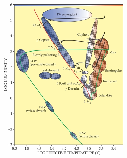
Typically, stellar models are evaluated by comparing their predicted paths through the HRD, indicated with black lines in figure 1, with the positions of actual stars in various stages of evolution. Evaluated by such basic criteria, the models have impressive strength. However, the evolutionary paths are appreciably affected by poorly known physical processes in the stellar interior, including convection, rotation, and the settling of atomic species. Early in their evolution, during their core-hydrogen-burning phase, stars with mass greater than about 2 M⊙ have a fully mixed, convective core and a diffusively mixed envelope in which radiative heat transfer dominates; for stars with mass less than about 1 M⊙, the core is radiative and the envelope is convective. (The exact cutoff values depend on a star’s metal content.) Stars of intermediate mass have a convective core and envelope separated by a radiative zone. (For more on stellar structure, see the article by Eugene Parker, Physics Today, June 2000, page 26 .)
After core-hydrogen burning, all stars have a convective envelope, but its extent is poorly known. Moreover, it’s possible that convection zones may arise at positions between the core and the outer envelope in some evolutionary phases.
In theory, a star’s internal structure can be inferred from its effective temperature and luminosity. But although Teff can be measured accurately from a stellar spectrum, L is notoriously difficult to determine; estimating L from measured fluxes requires precise knowledge of the distance between the star and Earth. For a limited number of relatively bright stars, interferometric measurements, 2 which combine the stellar light observed by an array of telescopes, have sufficient resolving power to deliver an estimate of R, which can in turn be used to determine L. (See the article by Theo ten Brummelaar, Michelle Creech-Eakmen, and John Monnier, Physics Today, June 2009, page 28 .) But for most stars, the uncertainties in L and other measurable surface quantities are too large to test predictions of interior phenomena.
In asteroseismology, mathematical models are used to relate periodic oscillations in a star’s brightness to perturbations in its internal equilibrium structure. The perturbed physical quantities—local pressure, density, temperature, luminosity, and combinations thereof—are expressed as a series of orthonormal eigenvectors. For a spherically symmetric star, a given quantity is described by the Lagrangian displacement vector ξ with components

where r is the distance from the stellar center, θ is the colatitude, and ϕ is longitude. The terms a and b are amplitudes, Ylm gives the spherical harmonics, and ωnlm is the mode’s angular frequency.
Each node lies along a concentric shell of constant r, a cone of constant θ, or a plane of constant ϕ. Three “quantum numbers” are therefore needed to specify each mode: The radial order n ≥ 0 gives the number of radial nodes; the mode degree l ≥ 0 specifies the number of surface nodes; and the azimuthal order m specifies how many of the surface nodes are along lines of longitude. (Likewise, l − |m| gives the number of surface nodes corresponding to lines of latitude.) It follows that −l ≤ m ≤ +l and that there exist 2l + 1 modes for each degree l. For a nonrotating star, the 2l + 1 multiplet components have equal frequency, but rotation lifts the degeneracy and gives rise to rotational splittings. 3
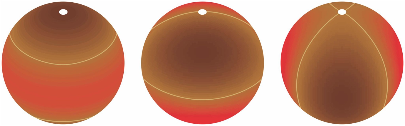
Figure 2 illustrates typical modulations in surface brightness for zonal (m = 0), tesseral (|m| = 1), and sectoral (|m| = 2) modes corresponding to quadrupole (l = 2) oscillations. In practice, we cannot spatially resolve the surfaces of stars as we can for the Sun. Instead, we detect fluctuations of the disk-integrated brightness over time, which reflects the simultaneous influence of all oscillating modes. The resulting light curves can fluctuate with amplitudes ranging from several parts per thousand (ppt) to parts per million (ppm) and frequencies ranging from a few microhertz to several thousand microhertz, depending on the type of star. 3 An example light curve, collected by the Kepler satellite from the star KIC 4726268, is shown in figure 3 along with its Fourier transform, which reveals the oscillation frequencies.

Figure 3. An asteroseismic portrait of the star KIC 4726268, as observed by the Kepler satellite. (a) An excerpt of the star’s light curve shows variations in the star’s disk-integrated brightness due to multiple seismic oscillation modes. (b) The Fourier transform of the light curve shows the oscillations in spectral form. In both panels, the deviation from the mean brightness is given in parts per thousand (ppt).
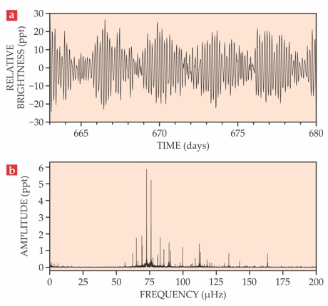

Figure 2. A simulated snapshot of an oscillating star’s quadrupole modes—a zonal mode (m = 0, left), a tesseral mode (|m| = 1, middle), and a sectoral mode (|m| = 2, right). The darker patches denote cool regions, the brighter patches denote hot ones, and the white dots denote the symmetry axes. Half an oscillation cycle later, the regions will have switched temperatures. Although surface brightness can’t be spatially resolved in actual observations, oscillation modes can be identified by the fluctuations they imprint on the disk-integrated brightness. The frequencies of those fluctuations can then be used to infer properties of the stellar interior.
To translate those oscillation frequencies into information about the stellar interior, one needs a forward seismic model—a model that takes the physical properties of a star as input parameters and predicts the star’s oscillations. Then, by finding parameters that yield oscillation frequencies ωnlm close to those observed, one can infer the properties of the observed star. The quantum numbers n, l, and m must be identified before any meaningful comparison between seismic data and model predictions can be made. That mode identification requires a physical interpretation of the measured frequencies.
Two kinds of quakes
From a physical point of view, oscillations can be categorized into pressure modes, restored primarily by pressure force, and gravity modes, restored primarily by buoyancy. Pressure modes, or p modes, correspond to acoustic waves propagating through the star’s envelope. They are the modes seen in the Sun, where their frequencies are in the range of 2000–4000 µHz. (For an overview of helioseismology, see the article by John Harvey, Physics Today, October 1995, page 32 .) Gravity modes, or g modes, on the other hand, correspond to internal gravity waves propagating through the radiative zones in the stellar interior.
The frequencies of a star’s g modes are typically a factor of 100 lower than those of its p modes. The spectral structures of the two kinds of modes don’t necessarily look different, but they can be distinguished by their respective frequency ranges, provided rough estimates of the stellar mass and radius are available. Theoretical models predict that beyond the core-hydrogen-burning phase, the density contrast between a star’s core and its envelope is large enough that the frequency ranges of p modes and g modes can overlap. As a result, some oscillations can simultaneously have p-mode character in the outer envelope and g-mode character in the core; such oscillations are therefore called mixed modes and hold particularly strong probing power throughout the entire star.
To interpret a frequency spectrum, it helps to understand the cause of the oscillations. We know of at least three excitation mechanisms. Cool, low-mass stars with convective envelopes—that is, solar-like stars and red giants—have p modes that are stochastically excited by turbulent convective motions. Such oscillations are continuously damped and reexcited and therefore have finite lifetimes ranging from days to months. Stochastically excited p modes have low disk-integrated amplitudes of tens of ppm or less, and their frequencies range from a few thousand microhertz for core-hydrogen-burning stars to a few tens of microhertz for red giants.
Most of the other types of oscillating stars exhibit self-driven, quasi-infinitely long lived modes excited by a heat-engine mechanism in opaque layers of partially ionized hydrogen, helium, or iron-like elements. The iron-like ions’ rich structure makes up for their low mass fraction; in hot stars, they can absorb sufficient heat to transfer radiative energy into oscillation modes. The heat-driven oscillations can have either p- or g-mode character and can occur across a wide range of luminosities and effective temperatures. They therefore span far larger ranges of amplitudes and frequencies than do stochastically excited p modes.
In a multiple-star system with stars orbiting each other at close range, stellar oscillations can also be excited by tidal forces. Those so-called forced oscillations may occur across the entire HRD, whenever the orbital frequency gets into resonance with g-mode frequencies; the observed frequencies are integer multiples of that orbital frequency.
By comparing the predicted oscillation properties of all the known classes of stars with the frequencies detected from KIC 4726268, a star having Teff of approximately 7000 K, we were able to deduce that it must be a so-called δ Scuti star exhibiting heat-driven p modes.
Taking the pulses of stars
The potential of asteroseismology to improve stellar evolution theory is ambitious but realistic. Oscillations can occur in every stage of a star’s life, and modern observational data reveal more oscillation modes than are predicted by computational modeling. That is not so surprising: To accurately predict a star’s excited modes, the star must be modeled in a nonadiabatic framework that includes an appropriate physical description of the stellar atmosphere. Because that undertaking is notoriously difficult, forward seismic modeling is usually done in an adiabatic framework, in which only the mode frequencies, not the amplitudes, must be identified. Just as in helioseismology, one usually fits the modes’ frequency differences—which are not subject to the uncertainties of the surface layers—rather than the individual mode frequencies. 4
In the case of p modes, a useful and easily measurable quantity is the large-frequency separation, the frequency difference between modes of the same degree but consecutive radial order. The large-frequency separation equals the speed of sound divided by twice the stellar radius and is closely related to the mean density of the star. The small- frequency separation, the frequency difference between one mode with radial order n and degree l and a second mode with radial order n − 1 and degree l + 2, is related to the sound-speed gradient. The small-frequency separation is a powerful diagnostic to estimate the age of a core-hydrogen-burning star, because its value is determined by the extent of the helium core, where the speed of sound is different from that in the hydrogen-rich near-core region. 1 , 3
For g modes, a natural diagnostic is the period spacing between low-degree modes of high, consecutive radial order. That spacing is related to the star’s internal buoyancy frequency and reflects conditions deep within the stellar interior. 3 Rotational splittings of the g-mode frequencies can reveal the star’s internal rotation frequency Ω(r). In fact, g-mode detection is currently the only method that can yield the full internal rotation profile of a star. (The internal rotation profile of the Sun, which does not exhibit g modes, was detected from the rotational splitting of p modes, 4 but only for r in the range 0.2–1.0 R⊙.)
Given the importance of internal rotation on angular momentum and chemical mixing, 1 a major quest of asteroseismology is to determine Ω(r) at the various stages of stellar evolution—particularly for stars with masses above about 8 M⊙, since those stars are responsible for the chemical enrichment of galaxies and the universe.
Aside from helioseismic treatments of the Sun’s thousands of p-mode oscillations, the first successes of asteroseismology were achieved via the ground-based Whole Earth Telescope (WET), a multisite photometric network enlisted to find white-dwarf oscillators in the early 1990s. Thanks to white dwarfs’ high-order g modes, which have large, ppt-level amplitudes and short oscillation periods, on the order of minutes, asteroseismology could be used to deduce the stars’ interior structure and global properties.
Just as helioseismology led to major improvements in the standard model of the Sun and of low-mass stars in general, 4 asteroseismology greatly refined models of the remnants of small stars. The best-studied case is the pre-white dwarf PG1159-035; 22 years of WET monitoring led to the detection and identification of 198 stellar oscillation modes, including some rotational splittings. Through seismic modeling, the WET team estimated the remnant’s mass to be 0.59 ± 0.02 M⊙ and its rotational period to be 1.3920 ± 0.0008 days. 5
Such results place strong constraints on the early evolutionary phases of a white dwarf’s progenitor star. For PG1159-035, they imply that the star must have started its cooling track with a helium-rich envelope of mass 0.017 M⊙. That places stringent limits on the mass lost due to dust-driven wind during the asymptotic-giant-branch phase, in which a carbon–oxygen core is enveloped by a shell of burning helium and hydrogen. During that phase, strong yet poorly understood chemical mixing makes a star’s evolutionary path highly uncertain. 6 The pre-white dwarf PG1159-035 was also shown to have rigid rotation, meaning it lost almost all of its angular momentum prior to becoming a white dwarf. 7
Into the space age
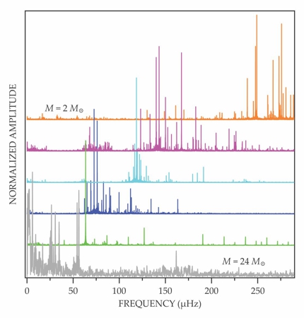
Although ground-based studies found oscillators in each of the classes shown in figure 1, the frequency spectra were noisy, which prevented the correct identification of many of the mode numbers n, l, and m. A breakthrough in asteroseismology of core-hydrogen-burning stars came from the uninterrupted, long-duration space photometry of the CoRoT and Kepler satellites. Figure 4 shows a sample of the oscillation spectra collected during the two missions.

Figure 4. Oscillation spectra of six stars—two, at bottom, measured by CoRoT and four, at top, observed by Kepler. All six stars are in the core-hydrogen-burning phase and oscillate primarily due to pressure waves excited by a heat-engine mechanism at work in the opaque gas layers. The stellar masses range from 24 M⊙ for the bottom star, for which 11 oscillation modes can be identified, to 2 M⊙ for the uppermost spectrum, for which hundreds of oscillation modes can be detected. Amplitudes have been normalized by the amplitude of the strongest mode in each spectrum and shifted vertically for visibility.
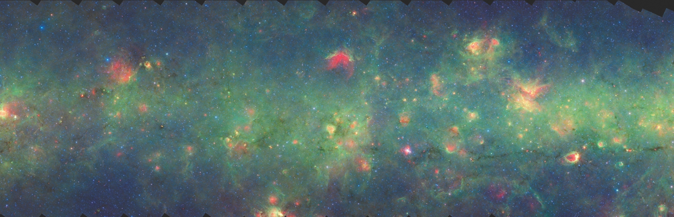
The CoRoT satellite monitored tens of bright stars for asteroseismology in addition to the thousands of faint, distant stars it observed in search of exoplanets. (For more on the search for exoplanets, see the article by Jonathan Lunine, Bruce Macintosh, and Stanton Peale, Physics Today, May 2009, page 46 .) Between 2006 and 2012, CoRoT’s telescope pointed toward either the center or the anticenter of the Milky Way and took measurements with 32-second integration during runs lasting 150 days for each field of view. The focus of CoRoT’s asteroseismology program was on massive stars ranging from 1.2 M⊙ to 60 M⊙, most having masses greater than 3 M⊙.

NASA/JPL-CALTECH/UNIV. OF WISCONSIN
Observations by CoRoT revealed unanticipated diversity in stars’ oscillatory behavior. The complex interplay of rotation, oscillation, binarity, and—for a minority of stars—bulk magnetism made it clear that rotation alone cannot explain the discrepancies between the theoretical models and the ppm-precision data. For 16 young blue stars with masses ranging from 3.2 M⊙ to 24 M⊙, seismic-modeling estimates of the masses of the convective cores indicated that the stars spend, on average, 20% more time in the core-hydrogen-burning phase than was predicted from previous models. 8
Kepler monitored some 150 000 stars in one field of view between 2009 and 2013. For part of that time, it monitored a few thousand targets with an integration time of 58.85 seconds per measurement and observed others using 29.4-minute integration times. The data for about 2000 solar-like stars led to the conclusion that they all have oscillatory behavior similar to that of the Sun and that their seismic behavior scales from the known helioseismic behavior as a function of two basic observables: the large p-mode frequency separation and the frequency of the maximum-power p mode. 3 Combined with a spectroscopic estimate of the effective temperature, those two observables give a solar-like star’s stellar mass, radius, and age with an average relative precision of 3.7%, 1.3%, and 12%, respectively. 9 (The calculated uncertainty takes into account uncertainties in the input physics of the models.) For individual solar-like stars modeled with high-resolution time-series spectroscopy or with a combination of interferometry and ppm-level space photometry, the uncertainties decrease typically by up to a factor of two. 10 Such high-precision detection of solar-like oscillations is of great benefit for the characterization of exoplanets, since the radius and mass of a transiting planet scale with those of the host star. And since asteroseismology can be used to determine the host star’s evolutionary phase, it provides a means to date exoplanet systems. 11
Kepler also observed thousands of red giants, following CoRoT’s discovery that they exhibit nonradial oscillations. 12 The Kepler data showed that such stars fulfill the scaling relations for solar-like p modes, which makes their distances and ages accurately determinable and therefore makes them suitable probes for galactic archaeology studies. 13 Kepler’s observations also led to the discovery of dipole mixed modes. 14 The simultaneous occurrence of mixed modes and p modes creates an opportunity to fit both the frequency separations and the period spacings of a star’s low-degree modes. Those quantities serve as excellent proxies for the star’s evolutionary phase and its progenitor’s path through the HRD. 15
There are three types of red giants: those that started the triple-alpha nuclear fusion process quietly, those that started it violently, and those still having a shrinking helium core surrounded by a hydrogen-burning shell. Distinguishing among them is impossible from their position in the HRD, since they have the same time-averaged surface properties. However, because their oscillations are affected by their quite different core and nuclear burning properties, the combination of mixed and p-mode measurements readily reveals their evolutionary phase.
Spinning stars
Within the “forest” of dipole mixed-mode frequencies detected in red giants 15 are both gravity- and pressure-dominated mixed modes. The former are more sensitive to the core properties than are the latter. In about 25% of the red giants monitored by Kepler, rotational splitting of the gravity-dominated mixed modes allowed the derivation of the core rotation frequency, plotted in figure 5 as a function of the stellar gravity g = GM/R2. Because a star’s radius grows and its gravity decreases as it evolves, stellar gravity is a proxy for evolutionary phase.

Figure 5. The rotation frequencies of solar-like stars are shown here as a function of stellar gravity g, which serves as a proxy for a star’s evolutionary phase. Blue indicates the core-hydrogen-burning phase; green indicates hydrogen shell burning with an inert helium core; red indicates hydrogen shell burning with a shrinking helium core; and orange indicates core helium burning. Envelope rotational frequencies are shown as triangles; core rotational frequencies are shown as circles. Rotational-frequency uncertainties are much smaller than the symbol sizes, and uncertainties in log g are typically around 0.1. (Figure constructed from data in B. Mosser et al., Astron. Astrophys. 548, A10, 2012
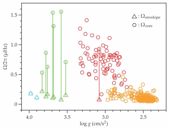
Astrophysicists were able to use rotational splittings of mixed modes to deduce the core and envelope rotation frequencies for seven single red giants and one primary of an eccentric binary. For two core-hydrogen-burning stars, the core and envelope rotation frequencies could be determined from separate, rotationally split p modes and g modes. Remarkably, asteroseismology has proven more successful than helioseismology in elucidating core rotation; the Sun’s core rotation is unmeasurable because its p-mode oscillations don’t probe the inner 20% of its radius.
The core rotation frequencies calculated for red giants are about two orders of magnitude less than current evolution models predict. That discrepancy can only be explained by an as yet undiscovered coupling between the core and envelope in low-mass stars during the hydrogen-shell-burning phase. Internal gravity waves excited by the convective core or by the hydrogen-burning shell could be a viable explanation. 16 Such waves were recently invoked by geophysicist Santiago Andrés Triana of the University of Leuven in Belgium to explain the counterrotation suggested by dipole g-mode splittings of the young, unevolved Kepler target KIC 10526294. Counterrotation in stellar interiors is still controversial, even though the phenomenon occurs frequently in planetary physics.
Whatever the true physical explanation of the data in figure 5, the seismic interpretation of the mixed modes in red giants is an important observational step toward improving stellar evolution theory of low- to intermediate-mass stars. It suggests that angular momentum transport begins earlier than thought and before the core-helium-burning phase.
A bright future
Although asteroseismology has been used extensively to deduce fundamental parameters of solar-like and red giant stars from scaling relations, its capacity to improve stellar models has by no means been fully exploited. The Transiting Exoplanet Survey Satellite and the repurposed Kepler spacecraft, K2, will open new avenues. 17 Despite their shorter observation times and K2’s less precise pointing, the new missions will observe regions of the sky—including young metal-rich star clusters, old metal-poor stellar clusters, and some of the biggest supergiant stars—that haven’t been seismically monitored and are highly relevant to galaxy evolution computations.
Following the recent discovery of a relationship between seismic oscillations and the star formation status, asteroseismology may also elucidate the periods just before and just after a star’s birth. 18 Asteroseismology of stars that have stopped accreting matter but have yet to achieve nuclear fusion in equilibrium will be of major relevance for the study of exoplanet formation. Exoplanet atmospheres may be seriously affected by the variability of their host star, and chemical modeling of the properties of the planetary atmosphere requires stellar models that take into account all relevant time scales. That is why the European Space Agency’s PLATO mission—which, after its launch in 2024, will characterize exoplanetary systems and look for Earth-like planets in habitable zones—has been designed to have full asteroseismic capabilities. It will observe some 1 million target stars from the second Lagrange point of the Sun–Earth system. 11
I gratefully acknowledge funding from the Research Council of the University of Leuven in Belgium and from the European Research Council. I thank my postdocs and PhD students for stimulating discussions and the staff of the Kavli Institute for Theoretical Physics at the University of California, Santa Barbara, for their kind hospitality.
References
1. C. J. Hansen, S. D. Kawaler, V. Trimble, Stellar Interiors: Physical Principles, Structure, and Evolution, 2nd ed., Springer (2004);
A. Maeder, Physics, Formation and Evolution of Rotating Stars, Springer (2009);
R. Kippenhahn, A. Weigert, A. Weiss, Stellar Structure and Evolution, 2nd ed., Springer (2012).2. A. Quirrenbach, Annu. Rev. Astron. Astrophys. 39, 353 (2001). https://doi.org/10.1146/annurev.astro.39.1.353
3. W. Unno et al., Nonradial Oscillations of Stars, 2nd ed., U. Tokyo Press (1989);
C. Aerts, J. Christensen-Dalsgaard, D. W. Kurtz, Asteroseismology, Springer (2010).4. J. Christensen-Dalsgaard, Rev. Mod. Phys. 74, 1073 (2002). https://doi.org/10.1103/RevModPhys.74.1073
5. J. E. S. Costa et al., Astron. Astrophys. 477, 627 (2008). https://doi.org/10.1051/0004-6361:20053470
6. A. H. Córsico, et al., Astron. Astrophys. 478, 869 (2008). https://doi.org/10.1051/0004-6361:20078646
7. S. Charpinet, G. Fontaine, P. Brassard, Nature 461, 501 (2009). https://doi.org/10.1038/nature08307
8. C. Aerts, Proc. Int. Astron. Union 9(S307), 154 (2014). https://doi.org/10.1017/S1743921314006644
9. W. J. Chaplin et al., Astrophys. J., Suppl. Ser. 210, 1 (2014). https://doi.org/10.1088/0067-0049/210/1/1
10. D. Huber et al., Astrophys. J. 760, 32 (2012). https://doi.org/10.1088/0004-637X/760/1/32
11. H. Rauer et al., Exp. Astron. 38, 249 (2014). https://doi.org/10.1007/s10686-014-9383-4
12. J. De Ridder et al., Nature 459, 398 (2009). https://doi.org/10.1038/nature08022
13. A. Miglio et al., Mon. Not. R. Astron. Soc. 429, 423 (2013). https://doi.org/10.1093/mnras/sts345
14. P. G. Beck et al., Science 332, 205 (2011). https://doi.org/10.1126/science.1201939
15. T. R. Bedding et al., Nature 471, 608 (2011). https://doi.org/10.1038/nature09935
16. C. Charbonnel, S. Talon, Science 309, 2189 (2005). https://doi.org/10.1126/science.1116849
17. S. Howell et al., Publ. Astron. Soc. Pac. 126, 398 (2014); https://doi.org/10.1086/676406
G. Ricker et al., J. Astron. Telesc. Instrum. Syst. 1, 014003 (2014). https://doi.org/10.1117/1.JATIS.1.1.01400318. K. Zwintz et al., Science 345, 550 (2014). https://doi.org/10.1126/science.1253645
More about the authors
Conny Aerts is a professor of astrophysics at the University of Leuven in Leuven, Belgium, and holds the chair in asteroseismology at Radboud University in Nijmegen, the Netherlands.


