Accelerating progress in climate science
DOI: 10.1063/PT.3.4772


Over the past 50 years, anthropogenic climate change has shifted from an abstract possibility predicted by a few scientists to a reality everyone can see and feel. Global-mean surface temperatures have risen 1 °C, and the Arctic has warmed a staggering 3 °C.

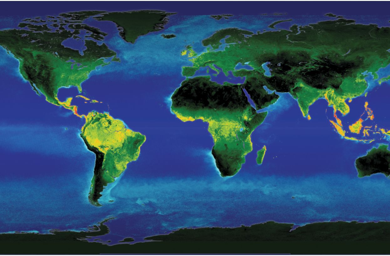
Satellite measurements of solar-induced chlorophyll fluorescence. Warmer colors show the locations with the most photosynthesis. (Courtesy of Philipp Köhler and Christian Frankenberg, Caltech.)
The principal cause is rising atmospheric carbon dioxide from the burning of fossil fuels. Transitioning to a low-carbon economy in the next several decades will be necessary to avoid catastrophic climate change that could, for example, push outdoor temperature and humidity in the Persian Gulf region beyond what humans can endure. 1 But even if societies succeed in bending carbon emissions downward, they will still need to adapt to climate changes that are already underway, including more severe heat waves, heavier rainstorms, and less summer irrigation water resulting from reductions in snowpack.
Adapting to that future requires accurate and actionable science. Although older and current climate models have predicted that Earth would warm and will continue to warm, projections vary greatly. For example, in scenarios in which CO2 emissions are promptly curtailed and ramp down to zero over the next 50 years, current models project that globally averaged surface temperature may still increase anywhere from 0.5 °C to 1.5 °C by 2050.
The large spread arises because of various uncertainties—such as how clouds respond to warming and how much heat oceans absorb—which are further compounded by the chaotic multidecadal variability of the climate system. Regional predictions are even more uncertain. And pinning down the shifting probabilities of extreme events, such as landfalling hurricanes or droughts, is still further out of reach.
A problem of scales
Together the atmosphere, land, oceans, cryosphere, and biosphere form a complex and highly coupled system. The fundamental laws governing the physics of the system are known, but the interactions of its many degrees of freedom exhibit emergent behavior that is not easily computable from the underlying laws.
The core challenge is to capture the Earth system’s great range of scales in space and time. Take cloud cover, a crucial regulator of Earth’s energy balance. The scales of its processes are micrometers for droplet and ice-crystal formation, meters for turbulent flows and convective updrafts, and thousands of kilometers for weather systems. Global climate models cannot resolve horizontal scales finer than about 50 km. Phenomena with smaller scales are represented by coarse-grained models, or “parameterizations,” which are systems of algebraic or differential equations that contain empirical closure parameters or functions to relate unresolvable processes to what is resolved. Biological processes, similarly, require coarse-grained models to connect what is known about the microscale biophysics of cells and plants to the emergent macroscale effects of heat stress or water limitation on tundra, tropical rain forests, and other biomes.
The traditional approaches to such multiscale problems are unlikely to yield breakthroughs when employed in isolation. Researchers have made deductive inferences from fundamental laws with some success. But deducing, say, a coarse-grained description of clouds from the underlying fundamental physical laws has remained elusive. Similarly, brute-force computing will not resolve all relevant spatial scales anytime soon. Resolving just the meter-scale turbulence in low clouds globally would require about a factor of 1011 increase in computer performance. 2 Such a performance boost is implausible in the coming decades and would still not suffice to handle droplet and ice-crystal formation.
Machine learning (ML) has undeniable potential for harnessing the exponentially growing volume of Earth observations that is available. But purely data-driven approaches cannot fully constrain the vast number of coupled degrees of freedom in climate models. Moreover, the future changed climate we want to predict has no observed analogue, which creates challenges for ML methods because they do not easily generalize beyond training data.
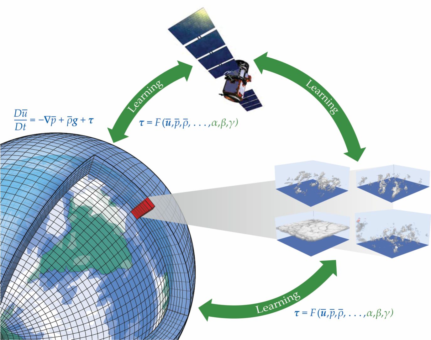
Dramatic progress may lie ahead by judiciously combining theory, data, and computing. Since the scientific revolution of the 17th century, the path to scientific success has been to develop theories and models, probe them through experiment and observation, revise them by learning from the data, and iterate. We believe that progress in climate science lies in a program that builds on that loop and accelerates and automates it with ML tools and high-performance computing, as illustrated in figure
Figure 1.

A loop connecting theory, data, and computing provides a framework to accelerate climate science. Theory yields the structures of coarse-grained models; in this case, it is the fluid-flow equations with an unknown closure function F. Learning from observations and local high-resolution simulations constrains unknown closure parameters and functions. Observations and local simulations target model weaknesses, and the cycle repeats. (Adapted from ref.
Advance theory
Parametric sparsity is a hallmark of scientific theories and is essential for generalizability and interpretability of models. For example, Newton’s law of universal gravitation has only one parameter, the gravitational constant. It replaced Ptolemy’s epicycles and equants, the deep-learning approach of its time. Ptolemy’s overparameterized model gave a good fit to the then-known planetary motions but did not generalize beyond them. The law of universal gravitation, by contrast, generalizes from planets orbiting stars to apples falling from trees. Because of its parametric sparsity, Newton’s theory produces trusted out-of-sample predictions, uncertainty estimates, and causal explanations.
Climate science needs to predict a climate that hasn’t been observed, on which no model can be trained, and that will only emerge slowly. Generalizability beyond the observed sample is essential for climate predictions, and interpretability is necessary to have trust in models. Additionally, uncertainties need to be quantified for proactive and cost-effective climate adaptation. Fortunately, the fundamental laws governing the microscale physical aspects of the climate system, including the quantum mechanics of radiation and molecules, the laws of thermodynamics, and Newton’s laws governing fluid dynamics, are well understood.
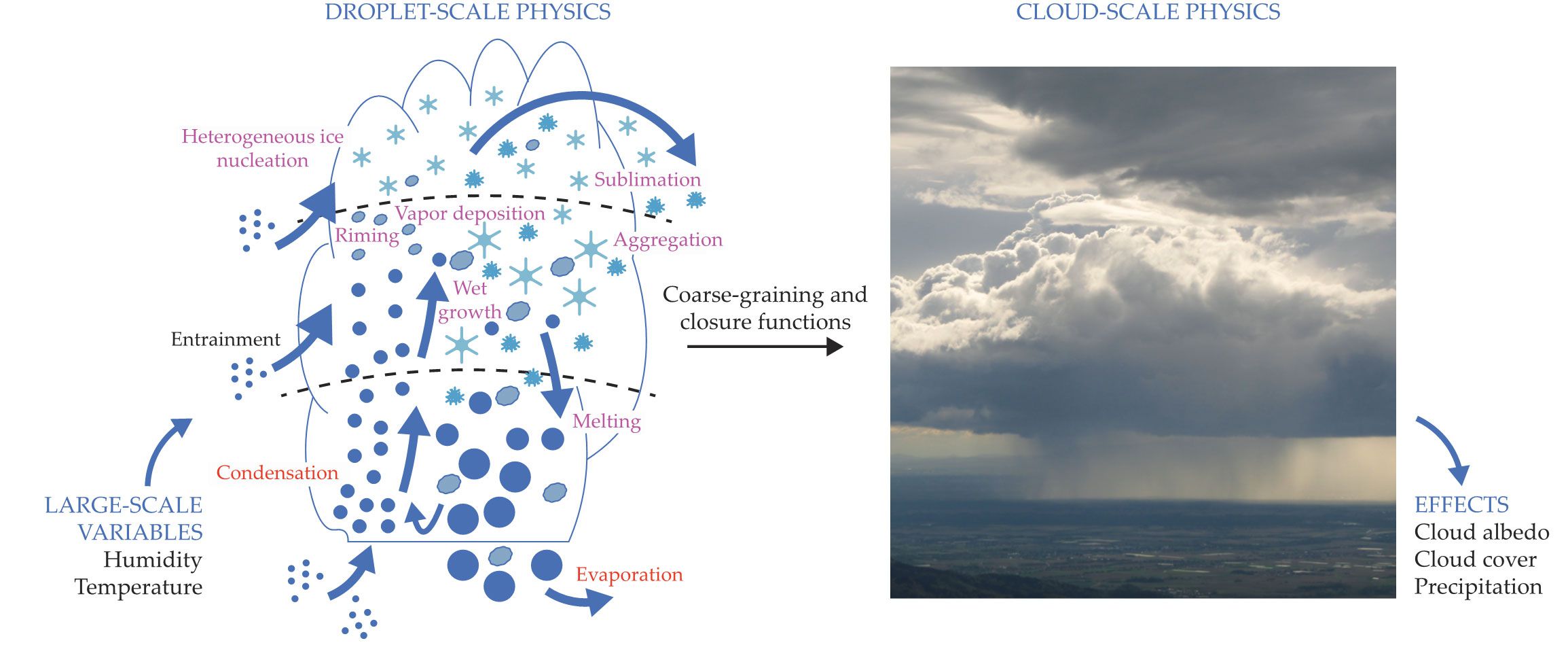
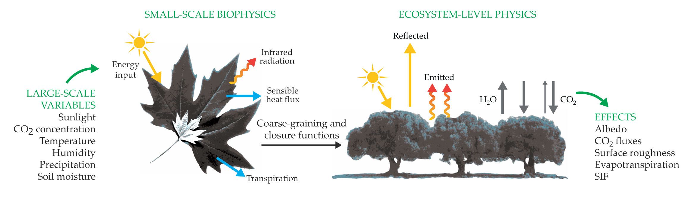
The task for physical theory is to coarse-grain the known microscale laws into macroscale models: By averaging over microscales, coarse-graining obtains models for the macroscale matched to the resolution of climate models. Processes that need to be coarse-grained for droplet-scale microphysics are illustrated in figure
Figure 2. Cloud microphysics parameterizations take in resolved values of temperature and humidity and then model the many unresolved interactions between suspended and precipitating cloud water and ice. The process produces as outputs precipitation and size distributions of cloud condensate, which determine cloud optical properties. (Left-hand image adapted from H. Morrison et al., J. Adv. Model. Earth Syst. 12, e2019MS001689, 2020, doi:10.1029/2019MS001689 ; right-hand photo by jopelka/Shutterstock.com.) Figure 3. Land biosphere parameterizations take in resolved variables such as temperature and sunlight and then coarse-grain processes such as plant hydraulics, transpiration, and photosynthesis. As outputs, they produce evapotranspiration, energy fluxes, and albedo, in addition to observables, such as solar-induced fluorescence (SIF), that are critical for closing the loop between models and observations. (Left-hand image adapted from Mostafameraji, CC BY-SA 4.0 ; right-hand image adapted from George Tekmenidis, CC BY-SA 3.0 .)

Researchers are pursuing new approaches, guided by systematic averaging and homogenization strategies, to model turbulence, convection, clouds, and sea ice, for example.
3
Empirical closure parameters and functions, which may be stochastic to reflect variability and uncertainty,
4
represent how smaller-scale phenomena affect the macroscale. Theory provides the structure of the coarse-grained models and closure functions and ensures, for example, the preservation of symmetries and conservation laws. But theory taken too far results in misspecified models that lead predictions and understanding astray. Where theory can go no further, closure parameters and functions must be inferred from data. The box on
Coarse-graining fluid equations
Theodore von Kármán deduced the “Law of the Wall” by averaging the Navier–Stokes equation for turbulent flows traveling past a wall. (See the article by Alexander Smits and Ivan Marusic, Physics Today, September 2013, page 25 .) Von Kármán decomposed velocity components parallel to the wall
The equation for
The theoretical reasoning underlying the Law of the Wall generalizes to the real atmosphere. Accounting for vertical density variations leads to Monin–Obukhov similarity theory, which is used to model near-surface turbulence in climate models. The theory contains an additional dimensionless height parameter and unknown functions of that parameter, which can be learned from data. In yet more complicated situations with nonlocal dependencies, such as atmospheric moist convection, theory may lead to systems of coarse-grained differential equations and closure functions that depend on functions of several nondimensional parameters. Such closure functions are natural targets for machine-learning approaches.
Harness data
Where theory reaches its limits, data-driven approaches can harness the detailed Earth observations now available. Often the data do not provide direct information about small-scale processes, such as in-cloud turbulence, that need to be represented in models. But the data do provide indirect information. For example, the observable distribution of liquid water and ice contains indirect information about in-cloud turbulence. Additional small-scale information can be generated computationally in high-resolution simulations for processes with known microscale governing laws, such as sea-ice fracture mechanics and convection and turbulence in the atmosphere and oceans.
Earth observations such as the energy fluxes at the top of the atmosphere are commonly used to calibrate models. What remains largely untapped, however, is the potential to discover and calibrate coarse-grained models by systematically harnessing all Earth observations jointly with data generated in high-resolution simulations.
Data-assimilation tools, used in weather forecasting for decades, and newer ML methods can be exploited for the task. For example, Bayesian approaches can be used to learn about closure parameters or functions, uncertainties, and errors in model structure. 5 ML emulators can greatly accelerate Bayesian learning, making it amenable to use with computationally expensive climate models. 6
Where model structures are unknown a priori, researchers may exploit data-hungry deep-learning approaches with proven scalability to high dimensions, or they may use sparsity-promoting discovery of coarse-grained models from dictionaries of differential-equation terms. 7 Whichever approach is pursued, preserving symmetries and conservation laws is essential, either bottom-up through the model structure or top-down through constraints on loss functions. Generalizability, interpretability, and uncertainty quantification remain crucial as well. 8 The field is ripe for experimentation and progress.
Leverage computing power
High-performance computing hardware is transitioning from architectures with central processing units to ones with graphics processing units (GPUs), tensor processing units, and other accelerators. To leverage the emerging architectures, climate models are being rewritten to an extent not seen in decades, to allow them to continue their march toward kilometer-scale resolution. As a result, the simulations of various phenomena, including monsoons and hurricanes, will improve. Simulations of rainfall will get more detailed, but they won’t necessarily become more accurate until Earth’s energy balance is captured correctly. That milestone will require more accurate simulations of low clouds and ocean turbulence. Those processes are out of reach in global models even at kilometer resolution.
Local simulations, however, can resolve smaller-scale processes whose governing equations are known. By capturing aspects of the present climate and climates for which there are no observed analogues, local high-resolution simulations can help prevent overfitting to the observed data. For example, clouds and the turbulence that sustains them can be simulated with meter-scale resolution in domains comparable to climate-model grid columns that are tens of kilometers wide. That approach suffices to resolve the most energetic turbulence, but smaller-scale phenomena, such as cloud microphysics, must still be represented by more uncertain coarse-grained models.
Isolated high-resolution simulations in a few locations have been used previously to calibrate cloud models, for example. Now massive cloud-computing resources (the other kind of cloud) make it possible to run thousands of high-resolution simulations concurrently. Automatically targeting the simulations to regions and seasons where they maximize information gain about a coarse-grained model is one way to close and accelerate the theory-data-computing loop. 9 The approach is similar to the ML paradigms of active and reinforcement learning, which have seen spectacular successes recently.
The theory-data-computing loop capitalizes on the successful methods of natural science. Theory directs data exploitation to areas where the science is most uncertain and provides model structures that are parametrically sparse, interpretable, and generalizable. ML tools and extensive computing accelerate the loop, potentially by orders of magnitude. This balanced approach to ML-accelerated science avoids the dual pitfalls of overreliance on reductionist theories for complex systems and overparameterization in purely data-driven, deep-learning approaches. The theory-data-computing loop requires a substantial initial investment in human and computational resources but results in climate models that, once calibrated with data, are computationally efficient and interpretable tools for prediction and scientific investigation.
To illustrate how ML-accelerated climate science may break new ground, consider three representative problems: How do atmospheric and oceanic turbulence, polar climates, and net carbon uptake by the land biosphere respond to climate change? Each of them responds strongly to the most familiar climate variation of all: the seasonal cycle. Seasonal variations in climate statistics—for example, temperature, sea-ice extent, and net carbon uptake—far exceed the climate changes expected over the coming decades. Some evidence suggests that seasonal variations are indicative of how the climate system may respond to the much slower greenhouse warming, apparently because similar mechanisms govern the response to seasonal insolation changes and longer-term changes in the concentration of greenhouse gases. Climate predictions may thus be improved by calibrating process-based models with the seasonal cycle.
Turbulence, convection, and clouds
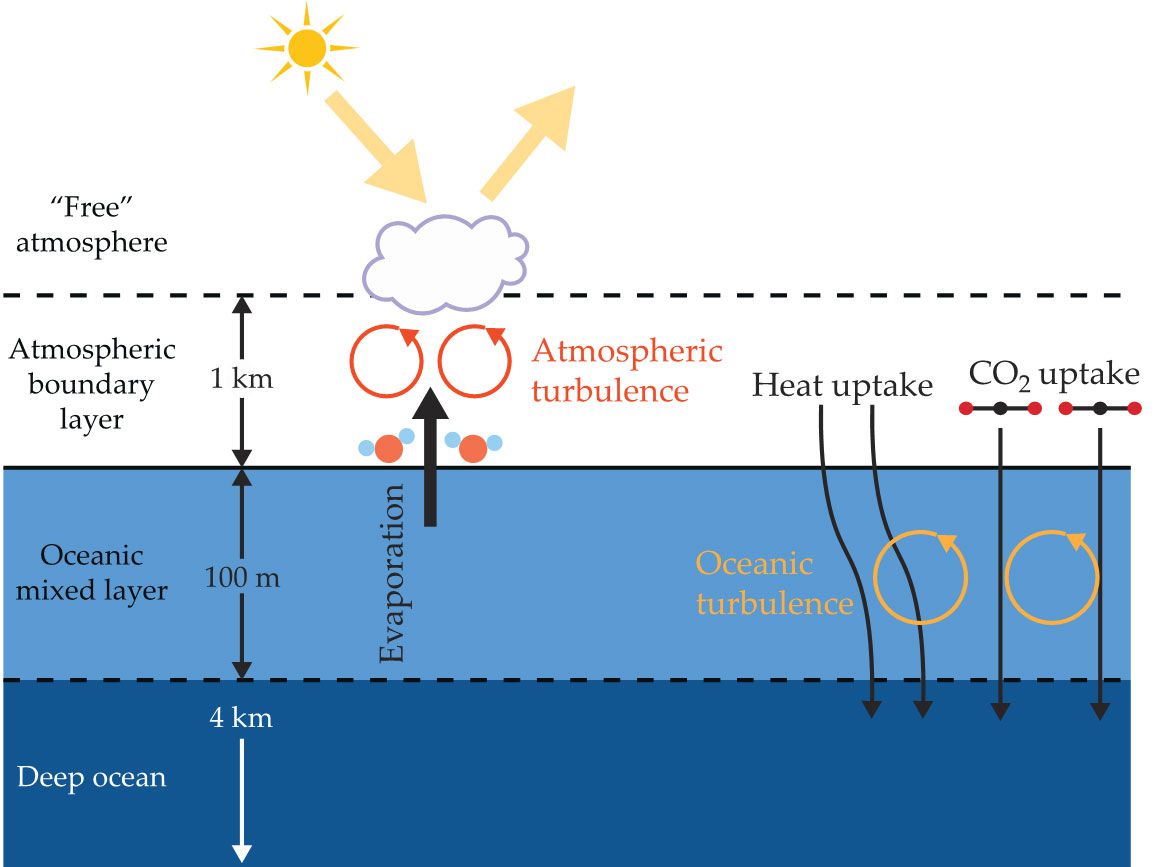
The principal sticking points in predicting climate are the subgrid-scale turbulent and convective motions in the oceans and atmosphere. In the oceans, the turbulent motions are the conduit through which momentum, heat, and tracers such as CO2 are transferred between the surface and the deeper ocean; they regulate the rate at which oceans take up heat and carbon. In the atmosphere, they transfer momentum, heat, and water vapor to and from Earth’s surface. They are critical for the formation of clouds, nourishing them with water vapor through convective updrafts. Figure
Figure 4.

Turbulence in the atmosphere and ocean connects the surface and the fluid interiors. Turbulent motions govern the sequestration of heat and carbon in the deep ocean and the transport of energy and water vapor into the atmosphere. (Illustration by Nadir Jeevanjee and Freddie Pagani.)
Clouds are the most visible outward manifestation of the turbulent and convective motions. They cool and warm Earth by reflecting sunlight and by reemitting some of the thermal IR radiation they absorb back to the surface, respectively. The net effect is that clouds cool Earth by 5 °C.
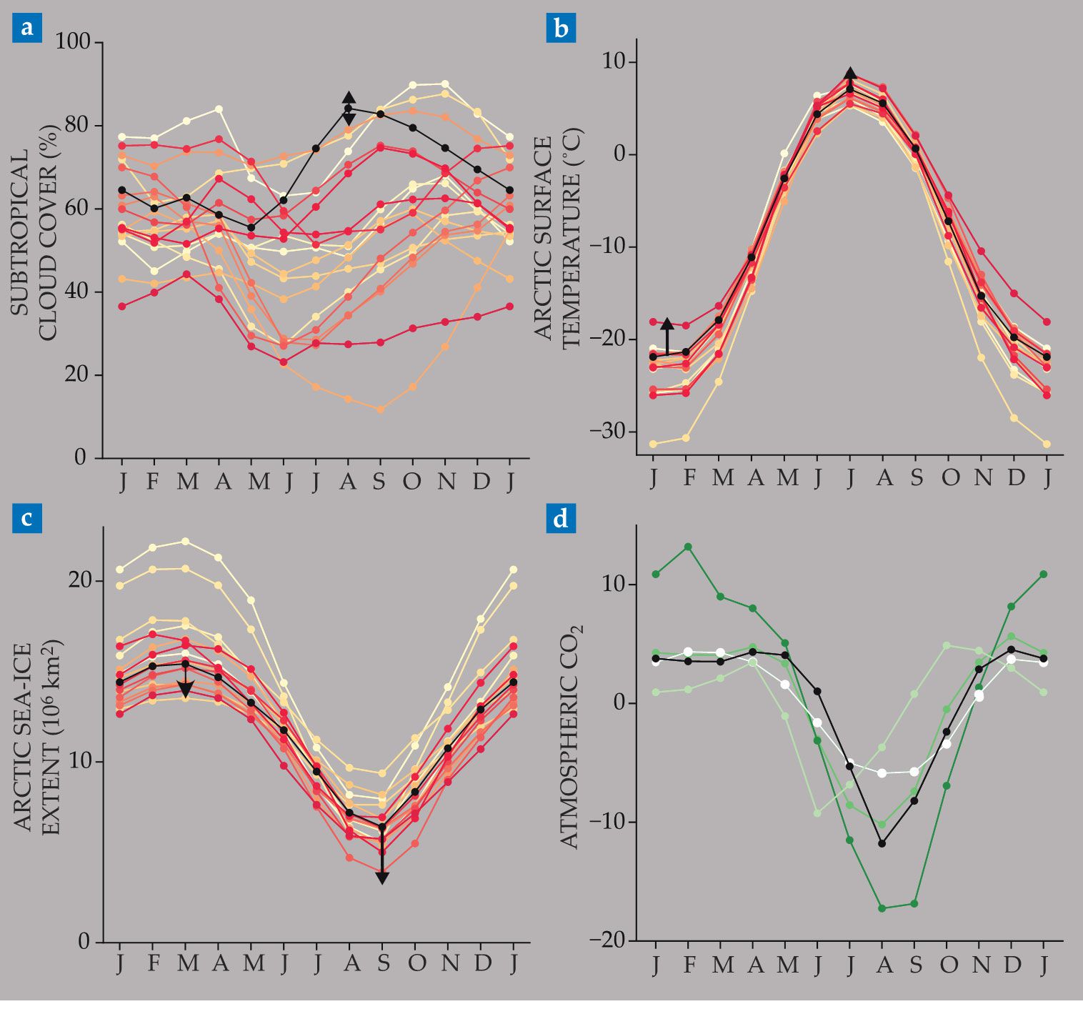
Simulated cloud cover often diverges widely from what is observed because the turbulent and convective motions that produce it are not well represented in models. For example, most models simulate fewer low clouds over subtropical oceans than are observed, and the seasonal cycle of cloud cover is likewise poorly captured, as figure
Figure 5.

Seasonal cycles (monthly data from January through January) in models (colors) and observations (black). (a) This plot shows cloud cover over the ocean off the coast of Namibia (10–20 °S, 0–10 °E). The models are colored from yellow to red in order of increasing climate sensitivity. (b) Similar to panel a, but this plot presents near-surface air temperature over the Arctic (60–90 °N). (c) Similar to panel b, but this plot shows Arctic sea-ice extent. The arrows in panels a–c indicate the magnitude and direction of the expected global warming response by 2050 under a high carbon dioxide emissions scenario; in panel a, the sign of the expected change is unclear. Models and observations in panels b and c are averaged over the years 1979–2019 (except for the cloud observations, which are averaged over 1984–2007). (d) Atmospheric CO2 concentration is shown as deviation from the annual mean for 1994–2005 at Point Barrow, Alaska.
The problem of simulating and understanding turbulence, convection, and clouds is well matched to the theory-data-computing approach. Recent theories have systematically coarse-grained the equations of fluid motion, be it by developing either separate equations for smaller-scale isotropic turbulence and convective updrafts or equations for statistical moments. In either case, the closure functions that represent processes such as turbulent exchange of fluid between cloudy updrafts and their environment are excellent targets for learning from data.
A similar approach that coarse-grains microphysical laws appears promising for the nonequilibrium thermodynamics that produces supercooled liquid cloud droplets, rather than ice crystals, at temperatures below freezing in rapidly rising updrafts. Nonequilibrium thermodynamics is responsible for the strong global warming response seen in some recent climate models. 10 Observations are particularly useful for providing information about coarse-grained models of cloud microphysics because the processes involved are not yet amenable to direct simulation.
Polar climates
All of the challenges that confound climate models play out simultaneously in polar regions. Turbulence in the often stably stratified polar boundary layer is intermittent and notoriously hard to model, and so are the clouds it sustains. The polar oceans are covered by sea ice, the extent of which depends on convection and clouds in the atmosphere above, turbulence and heat transport in the oceans below, and the nonlinear rheology of the ice itself.
In climate models, the amplitude of the seasonal cycle in Arctic temperatures can deviate several degrees from observations. As figure
Importantly, in simulations of recent decades, the amplitude of the seasonal cycle for Arctic temperature and sea-ice extent correlates with a model’s climate sensitivity—that is, the average warming after a sustained doubling of the CO2 concentration. More-sensitive models tend to have a lower seasonal-cycle amplitude and less sea ice. They are also more similar to observations than less-sensitive models, which bodes ill for the future of Arctic sea ice. Calibrating models with seasonal data is likely to make their predictions of polar climate changes more accurate.
Finely detailed space-based observations of polar cloud cover, distributions of sea ice, melt ponds on ice surfaces, and fractures in sea ice are now available. Autonomous robotic floats are beginning to give an unprecedented view of ocean properties and turbulence near the edge of and under sea ice, where warming waters are most effective at melting ice. The small-scale but important fluid dynamics of ocean waters under floating ice and along continental shelves is becoming amenable to local, targeted high-resolution simulations. Exploiting high-resolution simulations together with observational data much more systematically than has been done so far may bring the needed qualitative improvements in polar-climate modeling and prediction.
Land biosphere
Earth’s land biosphere removes about 30% of the human CO2 emissions from the atmosphere
11
(see the article by Heather Graven, Physics Today, November 2016, page 48 ). But how the land carbon sink changes as CO2 concentrations rise remains unanswered. Models differ widely in their simulation of past, present, and future carbon uptake. Consider, for example, the seasonal cycle of CO2 in high northern latitudes, which mirrors the seasonal cycle of boreal vegetation. Photosynthesis predominates during the growing season and draws carbon from the atmosphere. Respiration predominantes during wintertime and releases carbon back to the atmosphere. Figure
The discrepancies among seasonal cycles in the models percolate into the responses of the land carbon sink to rising CO2 emissions. Elevated CO2 concentrations fertilize plants by enhancing photosynthetic carbon uptake, unless water and nutrient availability limit the uptake. At the same time, increased temperatures enhance respiration and also affect photosynthetic uptake, which leaves uncertain the magnitude of the net effect of rising CO2 on the land carbon sink.
When the atmospheric CO2 concentration doubles, some models produce a global land uptake of 7% of the emissions (light green model in figure
The land biosphere’s net uptake of CO2 is the small residual of the much larger gross carbon fluxes associated with photosynthesis and respiration. Modeling progress has been hindered by poor knowledge of the gross fluxes. But new satellite data are upending the status quo. Soil moisture and vegetation cover are now being measured in unprecedented, hyperspectral detail. It has also become possible to estimate photosynthesis from space by measuring chlorophyll’s solar-induced fluorescence (SIF), which detects the excess near-IR solar energy that chloroplasts cast off during photosynthesis. 12 (See the opening image.) Combining satellite measurements of SIF and CO2 is now enabling scientists to disentangle the gross fluxes associated with photosynthesis and respiration.
Models of the biosphere are more difficult to design than models for physical aspects of the climate system. There is no straightforward way to coarse-grain the land or ocean biosphere. As a result, how to describe the biosphere is less clear: Should it be described at the level of genomes, plant functional types, biomes, or somewhere in between?
Nonetheless, the biosphere also obeys conservation laws, from energy to carbon mass, and small-scale processes—for example, photosynthesis, stomatal conductance, and plant hydraulics—are understood from first principles. The task for theory is to incorporate what is known on small scales into coarse-grained models that can effectively learn from data. Given the less-certain structure of biosphere models, ML techniques for data-driven model discovery, within the constraints of conservation laws, may improve biosphere models. Advances in computing and the use of GPU accelerators enable increased resolution and additional variables. A substantial improvement in land models can be anticipated, with the seasonal cycle as an obvious first target for model discovery and calibration.
Time for a broader effort
Our understanding of and ability to model clouds, polar climates, and the land carbon sink should improve substantially in the next decade. Ancillary benefits may be expected for activities such as seasonal to subseasonal prediction of extreme weather risks. Improved models and predictions of melting land ice, connected with sea-level rise, and of the deep-ocean circulation and its associated heat and carbon uptake may also be achievable. Reducing uncertainties in climate sensitivity by at least a factor of two may be in reach—a feat whose socioeconomic value is estimated to be trillions of dollars. 13
Paleoclimates that are the closest analogue of what awaits us are a natural next test for models of the climate system. The last time CO2 concentrations exceeded today’s level of 415 ppm was 3 million years ago, when Earth’s continental configuration looked as it does today but temperatures were 2–3 °C higher. 14 Cooling since then triggered the ice-age cycles, which are driven by variations in Earth’s orbit (see the article by Mark Maslin, Physics Today, May 2020, page 48 ). But it remains a mystery how the subtle orbital variations, amplified and modulated by feedbacks involving clouds, ocean turbulence, and the carbon cycle, work their way through the nonlinear climate system to produce the glacial–interglacial climate swings Earth has experienced.
Progress in one of the defining scientific challenges of our time requires well-funded collaborative teams with expertise ranging from the natural sciences—physics, biology, and chemistry—to engineering, applied mathematics, statistics, computer science, and software engineering. The rate of progress will be determined by the rate at which new talent joins the field. Come on in!
Many members of the Climate Modeling Alliance (CliMA.caltech.edu ), which is pursuing the approach outlined here, provided valuable feedback on drafts, as did Venkatramani Balaji and Mitchell Bushuk at the Geophysical Fluid Dynamics Laboratory and too many others to name here. David Bonan, Christian Frankenberg, Clare Singer, and Alexander Winkler made invaluable contributions of figures and data.
References
1. J. S. Pal, E. A. B. Eltahir, Nat. Clim. Change 6, 197 (2016). https://doi.org/10.1038/nclimate2833
2. T. Schneider et al., Nat. Clim. Change 7, 3 (2017). https://doi.org/10.1038/nclimate3190
3. V. Lucarini et al., Rev. Geophys. 52, 809 (2014). https://doi.org/10.1002/2013RG000446
4. T. N. Palmer et al., Annu. Rev. Earth Planet. Sci. 33, 163 (2005). https://doi.org/10.1146/annurev.earth.33.092203.122552
5. M. C. Kennedy, A. O’Hagan, J. R. Stat. Soc. B 63, 425 (2001); https://doi.org/10.1111/1467-9868.00294
A. M. Stuart, Acta Numer. 19, 451 (2010). https://doi.org/10.1017/S09624929100000616. E. Cleary et al., J. Comput. Phys. 424, 109716 (2021). https://doi.org/10.1016/j.jcp.2020.109716
7. S. L. Brunton, B. R. Noack, P. Koumoutsakos, Annu. Rev. Fluid Mech. 52, 477 (2020); https://doi.org/10.1146/annurev-fluid-010719-060214
S. H. Rudy et al., Science Adv. 3, e1602614 (2017); https://doi.org/10.1126/sciadv.1602614
W. E, J. Han, L. Zhang, https://arxiv.org/abs/2006.02619 .8. M. Reichstein et al., Nature 566, 195 (2019). https://doi.org/10.1038/s41586-019-0912-1
9. T. Schneider et al., Geophys. Res. Lett. 44, 12396 (2017). https://doi.org/10.1002/2017GL076101
10. M. D. Zelinka et al., Geophys. Res. Lett. 47, e2019GL085782 (2020). https://doi.org/10.1029/2019GL085782
11. T. F. Keenan, C. A. Williams, Annu. Rev. Environ. Resour. 43, 219 (2018). https://doi.org/10.1146/annurev-environ-102017-030204
12. G. H. Mohammed et al., Remote Sens. Environ. 231, 111177 (2019). https://doi.org/10.1016/j.rse.2019.04.030
13. C. Hope, Philos. Trans. R. Soc. A 373, 20140429 (2015). https://doi.org/10.1098/rsta.2014.0429
14. J. E. Tierney et al., Science 370, eaay3701 (2020). https://doi.org/10.1126/science.aay3701
15. A. J. Winkler et al., Nature Commun. 10, 885 (2019). https://doi.org/10.1038/s41467-019-08633-z
16. V. K. Arora et al., Biogeosciences 17, 4173 (2020). https://doi.org/10.5194/bg-17-4173-2020
More about the authors
Tapio Schneider is a professor of environmental science and engineering at Caltech in Pasadena, California. Nadir Jeevanjee is a physical scientist at NOAA’s Geophysical Fluid Dynamics Laboratory in Princeton, New Jersey. Robert Socolow is an engineering professor emeritus at Princeton University.


