Turbulence in two dimensions

Our world is largely made of fluids. Air and water are two of the most common materials on Earth, and their flow in the atmosphere and oceans determines weather and climate, among other things. On a less grand scale, engineered systems as varied as aircraft, industrial mixers, and pipelines involve the manipulation and control of fluid flow. Despite their differences, all those flows share a key feature: They are turbulent. Turbulence is, by and large, the normal state of fluid flow in the natural world and in engineering applications.

A crash course in turbulence

Precisely defining turbulence remains an open challenge, so I’ll have to settle for describing some of its many aspects. Turbulent flow is far from equilibrium and strongly chaotic. It is highly rotational, and it mixes and transports mass, energy, and momentum extremely efficiently. But perhaps the key feature of turbulence is that the flow is built from motions, often called eddies, that span a vast range of length and time scales. In the atmosphere, for example, eddies range from giant swirls spanning hundreds of kilometers down to tiny motions no more than a few millimeters across. The extent of that range is related to the well-known Reynolds number—the ratio of inertial to viscous forces. When the Reynolds number is large and inertial forces dominate, eddies of many scales are active and the flow is turbulent.

If all those eddies were more or less independent, as is the case in laminar flow, the fluid motion would be relatively simple to characterize and predict. Nature, however, has other ideas. The nonlinearities in the Navier–Stokes equations that govern fluid flow imply strong couplings between scales, so that energy and momentum are continually exchanged between eddies of different sizes. As a result, one can’t predict large-scale flow dynamics—for example, the average velocity field—without understanding the small scales, and vice versa.

Turbulence is both driven and damped; energy constantly flows into and out of the system. In a steady state, the rates of energy injection and dissipation must be the same. But the scales at which the two processes act are vastly different. The forces that drive the turbulence—things like gradients in solar heating of the atmosphere or fan blades in a wind tunnel—lead to the production of eddies at the largest turbulent scales. Turbulent energy is removed through viscosity, without which the energy injected into the flow would be conserved. In turbulent flows, however, viscosity is too weak to damp the large eddies; instead, it acts on very small-scale motions. Somehow, then, the system has to transport energy from large to small eddies.

As first conceived by British meteorologist Lewis Richardson and later made precise by Russian mathematician Andrei Kolmogorov, energy moves from large to small eddies via a cascade process: Large eddies spawn slightly smaller eddies, which in turn drive smaller ones, until finally, viscosity can do its job and turn the turbulent kinetic energy into heat. This idea of an energy cascade dominates the modern understanding of turbulence.

Two-dimensional turbulence

When turbulent flow is confined to a plane, the basic idea of an energy cascade still holds. Energy is injected at one scale and dissipated at another, with nearly lossless scale-to-scale transfer in between. Remarkably, however, in 2D turbulence, the direction of the cascade reverses; instead of cascading from the injection scale to smaller scales as in 3D, the energy moves to larger scales. What is it about changing the dimensionality that leads to such a drastic difference?

The answer is subtle, and the key lies with the vorticity, the curl of the velocity field. The vorticity gives the local angular velocity of the fluid; when it is large, the fluid is more rotational. The square of the vorticity, called the enstrophy, measures the local strength of the rotation. In 3D, the total enstrophy in the flow (that is, the volume integral of the enstrophy) can change in two ways. Just as for energy, it can be dissipated by viscous effects. But even absent viscosity, enstrophy can change via a process called vortex stretching. If a vortex is pulled tight along its axis, its rotation rate and therefore its enstrophy will increase, much as the frequency of a wave on a string increases when the string is put under tension. The forces required to pull on the vortex can come from the flow itself.

In 2D, however, vortex stretching can’t happen; there is no axis perpendicular to the vortex on which to pull! As a result, total enstrophy, like energy, is conserved in 2D flows without viscosity.

The arguments for the energy cascade in 3D turbulence apply equally to enstrophy in 2D turbulence. And indeed, experiments have observed a cascade of enstrophy from large scales to the small scales at which it is dissipated by viscous forces. Energy, however, is a different story. The rate of energy dissipation is determined by the product of the viscosity and the enstrophy, as can be derived from the Navier–Stokes equations. Surprisingly, in 3D the energy dissipation is independent of the viscosity even in the limit of very small viscosity; the decrease in viscosity would be balanced by an increase in enstrophy due to enhanced vortex stretching. In 2D, however, vortices don’t stretch, and so the rate of energy dissipation vanishes as the viscosity goes to zero—or, equivalently, when the Reynolds number is high and the turbulence is strong.

That result poses a conundrum: Viscosity doesn’t dissipate energy in strong 2D turbulence, but if the energy winds up in small eddies via a cascade, it will surely be removed by viscous forces. The way out is that energy doesn’t cascade to small scales in 2D. The planar flow is still turbulent, which implies that the energy should flow away from the forcing scale due to nonlinear effects. But since it can’t go to small scales, it must flow to large eddies in what is known as the inverse cascade. In theory, the eddies generated by the inverse cascade can be as large as the system itself.

The inverse cascade has numerous implications that make 2D turbulence very different from its more common 3D counterpart. The usual 3D turbulent flow appears to be the epitome of randomness; it is extremely chaotic, and the dynamical variables exhibit frequent, unpredictable, and violent fluctuations. The energy cascade continually pumps energy into small eddies, which leads to large gradients in the velocity field. But in 2D, the inverse cascade drives energy into spatially smooth, large eddies, thereby enhancing spatial coherence by smoothing out small-scale variability. Thus, whereas turbulent flows in 3D are largely incoherent, 2D turbulent flows strongly tend to self-organize and form long-lived, large-scale dynamical structures. The tendency of the inverse cascade to drive energy into such large-scale structures, a phenomenon called “spectral condensation,” is strikingly similar to Bose–Einstein condensation in atomic systems and can also be related to a number of problems in plasma physics in which dynamics of the flow lead to spontaneous ordering.

Real-world applications

It might seem that studying 2D turbulence is simply an academic exercise because true 2D flow only exists in a theorist’s brain or on a computer. But the phenomenology of 2D turbulence is remarkably robust. Controlled experiments, real-world observations, and recent theory all suggest that perfect two-dimensionality is not a necessary condition for an inverse energy cascade to exist. In fact, the theory of 2D turbulence has applications to a surprisingly wide range of real-world systems.

It is no accident that the meteorology community was the first to study 2D turbulence. The atmosphere is very thin compared with its lateral extent. Motion in the lateral direction is much less constrained than in the vertical direction, and 3D effects are significant only at small scales or near boundaries. Planetary rotation tends to suppress vertical flow, as does vertical density stratification in, for example, bodies of water (see the Quick Study by Jeff Carpenter and Mary-Louise Timmermans in PHYSICS TODAY, March 2012, page 66 ). On large scales, the atmosphere and sea behave roughly as 2D flows.

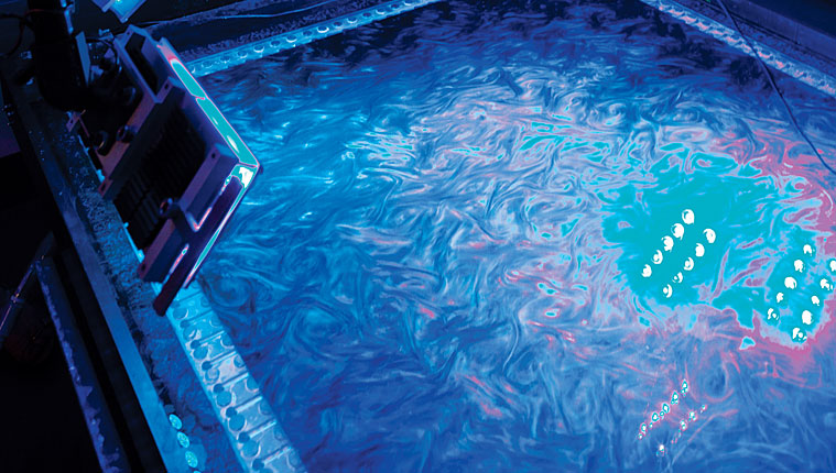
Laboratory experiments to study 2D turbulence typically look at flowing soap films or, as shown in the figure, a thin layer of conducting fluid stirred by electromagnetic forces. The intensity of the turbulence in the experiments can be pushed only so high; if, for example, the conducting liquid is stirred too vigorously, the system will develop significant 3D flows. Nonetheless, such studies of 2D turbulent flow have helped physicists develop an understanding of this complex dynamical system.

Although the basic phenomenology of 2D turbulence is understood and accepted, many of its details remain to be worked out. Of particular concern are the interactions by which eddies exchange energy in the inverse cascade; theory predicts them to be rather different from interactions for 3D turbulence. A second topic of interest is the feedback between the large eddies generated via the inverse cascade and the rest of the turbulence. No doubt plenty of surprises lie on the horizon.

References

1. G. Boffetta, R. E. Ecke, “Two-dimensional turbulence,” Annu. Rev. Fluid Mech. 44, 427 (2012). https://doi.org/10.1146/annurev-fluid-120710-101240
2. R. H. Kraichnan, D. Montgomery, “Two-dimensional turbulence,” Rep. Prog. Phys. 43, 547 (1980). https://doi.org/10.1088/0034-4885/43/5/001
3. R. H. Kraichnan, “Inertial ranges in two-dimensional turbulence,” Phys. Fluids 10, 1417 (1967). https://doi.org/10.1063/1.1762301
More about the authors
Nick Ouellette is an assistant professor in the department of mechanical engineering and materials science at Yale University in New Haven, Connecticut.