How to measure earth’s magnetic field

Magnetic measurement is an old science, but it’s one that continues to be of tremendous importance. The compass is a familiar magnetometer that indicates the horizontal component of the ambient magnetic-field vector. Magnetic measurements today are accomplished by a wide variety of magnetometers, usually coupled to digital data-acquisition systems. The article by Jeffrey Love on page 31 describes the many applications of magnetic-field measurements made at terrestrial observatories. Most often used for geomagnetic measurements are the fluxgate magnetometer, which gives vector components, and the proton precession magnetometer, which measures field intensity.

Fluxgate magnetometer

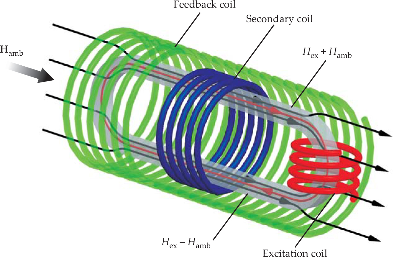
Figure 1 illustrates the essential elements of a fluxgate magnetometer. As in a transformer, a soft magnetic core is surrounded by both a primary and a secondary coil. The primary, or excitation, coil induces a field in the core; the secondary measures the core’s response.

When a weak field H is applied, the magnetic induction B ≡ μ H exhibits a linear response. Here, μ is the permeability. In principle, μ depends on the field strength, but for weak fields, it is constant. Passive search coil magnetometers and AC-driven transformers work in the linear regime.

The fluxgate magnetometer, by contrast, is subjected to an alternating excitation field H _ex large enough to saturate the core at a constant value of B. Due to the nonlinear characteristics of the core material, the signal induced in the secondary coil would be expected to include oscillations of odd multiples of the excitation frequency—in other words, odd harmonics. Absent an ambient field H _amb, no even harmonics would be present. Earth’s ambient field, however, disturbs the symmetry of the core field and leads to a signal in the secondary coil with even harmonics of the excitation frequency. The amplitudes of those even harmonics are proportional to the component of ambient field parallel to the secondary-coil axis. If the secondary coil is wrapped around the two core elements with opposite excited flux, as in figure 1, the odd harmonics of the induced voltage vanish and leave only the harmonics that depend on the ambient field.

The field measurement can be realized as a current measurement. A feedback coil compensates the ambient field at the core position; the required current is proportional to the magnitude of the field.

In 1936 Hans Aschenbrenner and Georg Goubau published the first fluxgate sensor design. They used a ring core made with a bundle of soft iron florist’s wire and achieved a resolution of better than 1 nanotesla. In the following years, fluxgate magnetometers were developed primarily for industrial and military purposes. Soon after World War II, however, geophysicists began to use them to investigate Earth’s magnetic field. Slowly, fluxgate magnetometers replaced the classical variometers that used suspended and balanced magnets.

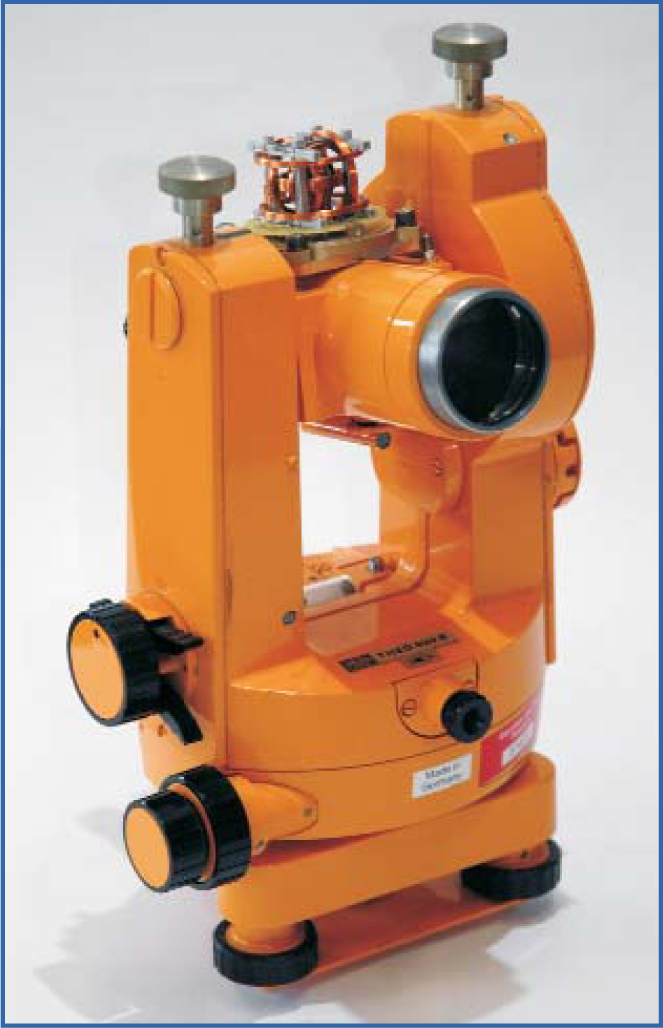
Fluxgate magnetometers can achieve a resolution of about 0.01 nT for magnetic-field components with frequencies in the range of 0–100 Hz. But magnetometers that operate continuously, such as those at magnetic observatories, are subject to offset drift, so their baseline has to be corrected. To do that, a fluxgate sensor is mounted parallel to the telescope axis of a nonmagnetic theodolite. (A theodolite is a device with a rotatable telescope; surveyors commonly use them.) Figure 2 shows the apparatus that, since 1970, has become a standard instrument for observation of the geomagnetic-field direction.

The fluxgate technique has many applications outside the geomagnetic observatory. A fluxgate magnetometer built by Shmaia Dolginov and flown aboard Sputnik 3 in 1958 was one of the first scientific instruments in space. Almost all subsequent space missions investigating the geomagnetic field, Earth’s magnetosphere, or the solar system have been equipped with fluxgate magnetometers. But fluxgates aboard vessels and aircraft or along the sea floor are also used in a variety of studies closer to home.

Proton precession magnetometer

The discovery of the relation between proton precession and magnetic-field intensity had important ramifications for the field of magnetic measurement. All nuclei that contain odd numbers of protons have an intrinsic magnetic moment μ and angular momentum L related by μ = γ L. The proportionality constant γ depends on charge and mass only; for protons, the value of that gyromagnetic ratio is γ = 267 515 528 Hz/T. If a proton is exposed to a constant B, it behaves like a spinning top in a gravity field and experiences a torque T = d L/dt = μ × B. The consequence of this dynamical equation is that L precesses around B with the Larmor frequency ω = γB. Thus the value of B can be deduced from a frequency measurement; for the first time, the field could be related to a physical constant independently of environmental conditions. The proton precession magnetometer is the tool of choice for most magnetic surveys made for exploratory purposes. In such cases scalar information is sufficient. And a scalar-only survey is much easier to conduct than a full vector mapping.

In practice, a coil wound around a bottle containing water, alcohol, or some other fluid with a large number of protons induces a large field that polarizes the protons and gives them a net magnetization. That same coil can be used later for the frequency measurement. To achieve a maximum signal in the coil, the polarization direction should be oriented approximately perpendicular to Earth’s magnetic field. After the polarization field is abruptly switched off, the magnetization vector precesses around Earth’s field and induces a signal at the Larmor frequency, about 2000 Hz. The measurement period is limited to 1 second or so because the signal amplitude decays exponentially with time, and both local and temporal field gradients accelerate the decay. Moreover, the signal is weak, and the precession frequency has to be measured with an accuracy of one part in 10^5. Thus one needs sophisticated electronics to condition the signal and increase frequency resolution.

Felix Bloch described the fundamentals of nuclear induction in 1946. He and Edward Mills Purcell were awarded the 1952 Nobel Prize in Physics “for their development of new methods for nuclear magnetic precision measurements and discoveries in connection therewith.” By the late 1940s, geophysicists could avail themselves of the first precession-based instruments for measuring the intensity of Earth’s magnetic field. By 1960 magnetic observatories had also begun to use them.

The introduction of the proton precession magnetometer was a milestone in field-intensity measurements. The intensity, which until then was the weak point of the vector measurement, could now be determined with an accuracy of about 1 nT. A further improvement was the development of the Overhauser magnetometer, which afforded continuous and more effective polarization. In that instrument, unbound electrons are exposed to an RF field and transfer their excitation energy to protons. That technique allows the sampling rate to be increased by an order of magnitude, to about 5 Hz. Nevertheless, proton precession magnetometers have their shortcomings. For example, their operation requires homogeneous fields with magnitudes greater than 20 000 nT.

Although the basic proton precession magnetometer described above measures field magnitude only, it is possible to determine field components with a modified design. If the sensor is equipped with coils that generate bias fields, one could run a pair of measurements in which the bias fields are applied in opposite directions. That is, one can measure $\left|{\text{B}}_{\text{Earth}}\hspace{0.17em}\pm \hspace{0.17em}{\text{B}}_{\text{bias}}\right|$ . Subtracting the squared magnitudes yields the component of Earth’s magnetic field in the bias-field direction. That variometer mode and the simpler intensity-only mode are the main applications of proton magnetometers in magnetic observatories.

An important thrust of current research is to automate the magnetic observatory by combining fluxgate or proton precession magnetometers with optical instruments. Nonmagnetic mechanical systems under development would rotate the magnetometers and optical sensors to eliminate error sources and allow for absolute measurement of the geomagnetic field at regular intervals. At present, such systems are prototypes. If, however, an automated system should prove reliable, it could open the door to a more uniform worldwide distribution of magnetic observatories.