Hip bone is connected to … II

In a previous column (Physics Today, September 2005, page 10 ), I indicated how computer models might be used to mimic and describe a few of the small networks that control and drive biological systems. I focused on the understanding that could be obtained from moderately accurate descriptions of relatively simple biological systems. Here I look at conceptualizations of much larger networks. (See also the article by Mark Newman, Physics Today, November 2008, page 33 .)

Forty years ago Stuart Kauffman took on the immensely challenging task of understanding something about the interlinked chemical activity in a living cell. He despaired of the task of doing the problem in anything like its full detail but instead decided to describe it by a vastly simplified and generalized model. He started with N variables or “nodes,” each representing a chemical species that might be present in a cell. ¹ The possible states of the cell were specified by snapshots that described each species as present or absent at a given time. The cell dynamics was a vastly simplified, stepwise process. Each compound’s presence at time t + 1 depends on the presence or absence of a few other compounds at time t. Thus, for example, compound A would be present at time t + 1 if B and C were present at time t but D was absent. Kauffman described the entire biological cell by listing rules like that one for all the N compounds in the cell.

The rules are largely built into the DNA and the structure of the cell so that the rules remain largely fixed through many cell divisions.

Of course, one could invent a huge number of networks that would fit the description of a cell. Different networks would be specified by giving different connections and different rules for the formation of each particular chemical compound. The task of finding the rules for a given biological system could be expected to be immense, providing a job for more than one generation of biochemists and biologists.

Kauffman was unwilling to wait. Instead he built upon work of Paul Erdös and Alfréd Rényi, in which they studied ensembles constructed from all possible networks of a given type. ² Two parameters would describe the average properties of the biological cell: the number of compounds, N, and the average number of precursors, K, whose presence or absence would determine the formation of a given compound. Kauffman picked at random from all possible networks with given N and K, asking what could be learned by saying that biological systems are constructed from a “typical” set of rules. ¹ His approach is somewhat similar to the Boltzmann–Gibbs strategy for statistical mechanics, which says that a configuration for a set of gas molecules might be described as picked at random from all possible configurations of N molecules with a given energy.

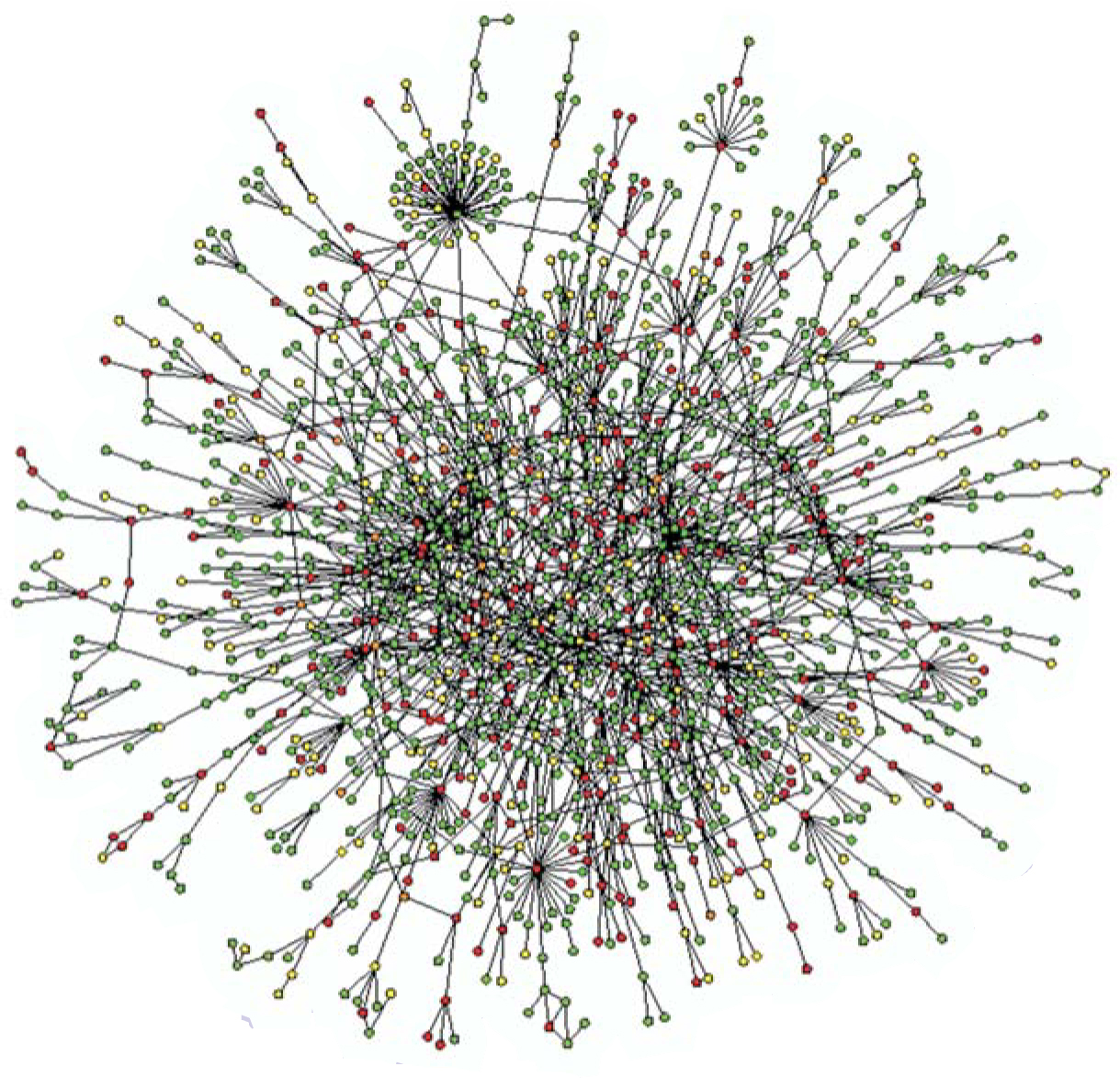
In recent years people have learned the detailed structure of such networks for a few biological systems by painstaking experimental study of all their reactions and interactions. A lot can be learned from examining such specific examples. Figure 1 shows one such network. But it is also interesting to look back and see what has been learned from the general features of Kauffman’s analysis. Because each compound may be either present or absent, the number of configurations is 2 ^N , so that eventually the cell must return to a configuration it has visited earlier. Because the time-development rules are fixed, thereafter the cell can only retrace its earlier steps. Thus the system will eventually settle down into a repetitive, cyclical behavior. A given system can support several different repetitive cycles so that, depending on initial data, the cell will fall into one of several cycles. Kauffman took the different cycles to each represent a different kind of cell. Our bodies contain many different cell types—skin, brain, muscle … each with an identical genetic makeup. Just as different cycles of dynamical systems might be generated by giving the systems different initial conditions, so different cell types emerge from identical dynamics but different starting conditions.

One might begin to ask about the generic properties of such networks. For an overview of the work done, see the review paper of Max Aldana, Susan Coppersmith, and me. ³ One of three kinds of behavior can be discerned in a given network. If the connections among nodes are sparse, different parts of the system each have their own dynamics independent of the other parts. For such systems, which arise when the average K is less than 2, we get a kind of frozen behavior in which there is too little linkage among the different nodes for the system to exhibit the types of complexity characteristic of actual biological situations. Conversely, for K greater than 2, the network motion is totally chaotic in that a change in the rule at almost any node can change the subsequent behavior in a finite fraction of all the nodes of the system. Such a structure is much too noise-sensitive to represent the noise-tolerant response characteristic of real biological systems. For K very close to 2, the system displays a kind of critical behavior intermediate between frozen and chaotic states. In that case a change in an initial value of a node or in the rule for updating a certain node causes a small subset of the nodes to change their behavior. However, most of the nodes will continue to follow the same pattern as before. That kind of partially flexible, but mostly unchanging, behavior is characteristic of most biological systems. Biologists describe such behavior by using the word “robust.”

Kauffman thus argued that biological systems might well show a kind of critical dynamics, akin to the dynamics seen near the critical point of a phase transition. Nowadays that argument is widely accepted as giving a very rough but reasonable result.

Detailed study of networks

In recent years biologists have been able to see the actual dynamics of a few much-studied networks. Each of those networks had previously been analyzed piece by piece in experimental work by biochemists and biologists. The nodes each contain the concentration of the different chemical compounds. Each node is linked to the compounds that determine its production rate. Such studies do not support the initial presupposition that biological networks look like they have been picked from a randomly constructed ensemble. Indeed, many of the networks have been understood as being structured from small pieces that provide rather elementary functions, like the AND and OR gates found on a computer chip. (See, for example, René Thomas’s extensive analysis of the component pieces of biological networks. ⁴ )

Furthermore, recent work has shown that many biological networks are constructed from a few preferred small structures. Uri Alon and his coworkers have analyzed small pieces—containing only a few nodes and their interconnections—carved from large biological networks, and they have counted the frequency of occurrence of the different possible structures. ⁵ They then compared these frequencies with ones drawn from randomly connected networks, à la Kauffman. The biological networks showed a detailed structure quite different from the purely random systems. In particular, in each network a few of the structures, called motifs, appeared far more frequently than one would expect from randomness.

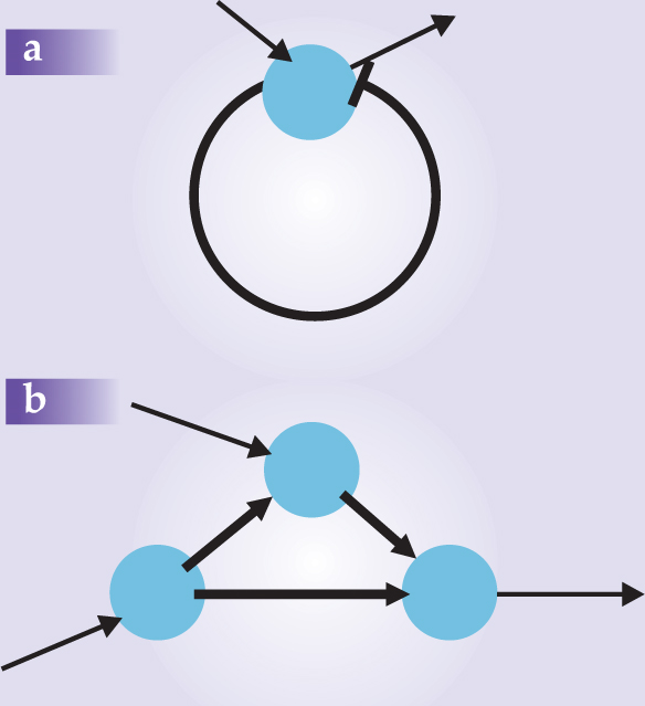
For example, according to Alon, in contrast to a random network, there are many more negative feedback loops with the structure of figure 2 than one might expect at random for a network characterized by an average connectivity, K. The negative feedback loops act as “thermostats,” which can control in a precise and reliable manner the concentration of important chemical species. In contrast, the number of positive feedback loops is far smaller because biological systems have little use for runaway quantities.

Different biological networks have different motifs because different kinds of small structures might serve useful purposes in each context. Evolution will then especially select those structures that are robust—that is, those that maintain their functionality even when changed slightly. Alon further argues that evolution, like a computer programmer, tends to duplicate and reuse structures already proven to be useful. So he expects that each kind of network will show its own list of oft-repeated motifs.

Thus recent studies move far from Kauffman’s random networks. However, the randomness is not the important take-home message from the earlier work. Rather, the enduring point is the three states of the system—frozen, critical, and chaotic—and the contrast between the way information flows in each state. This message is far broader than the model that originally supported it and is used in many different areas of physics, mathematics, and computer science. The change between the ordered and chaotic modes is called the percolation transition and is a ubiquitous descriptor of the slow transfer of information.

References

1. S. Kauffman, J. Theor. Bio. 22, 437 (1969).https://doi.org/10.1016/0022-5193(69)90015-0
2. P. Erdös, A. Rényi, Publ. Math. 6, 290 (1959).
3. M. Aldana, S. Coppersmith, L. P. Kadanoff, in Perspectives and Problems in Nonlinear Science: A Celebratory Volume in Honor of Lawrence Sirovich, E. Kaplan, J. E. Marsden, K. R. Sreenivasan, eds., Springer, New York (2003), p. 23.
4. R. Thomas, personal web page, http://www.ulb.ac.be/cenoliw3/PERSO-PAGES/rthomas.html .
5. U. Alon, An Introduction to Systems Biology: Design Principles of Biological Circuits, Chapman and Hall/CRC, Boca Raton, FL (2007).
More about the authors
Leo Kadanoff (leop@uchicago.edu ) is a condensed-matter theorist at the University of Chicago.
Leo P. Kadanoff, (leop@uchicago.edu) University of Chicago .